Vignette: Estimation of total copy numbers using the CRMA v2 method (10K-CytoScanHD)
Author: Henrik Bengtsson
Created on: 2008-12-09
Last updated on: 2014-12-21
This document describes in detail how to estimate total copy numbers (CNs) in aroma.affymetrix according to the CRMA v2 method described in Bengtsson, Wirapati, and Speed (2009). All the steps of CRMA v2 will be done one by one and the output of each step will be discussed. If you wish to run CRMA v2 without going through the details, see the doCRMAv2() function, which wraps up all of the below in one call.
The CRMA v2 method is a preprocessing and probe summarization method that provides full-resolution raw total copy-number estimates, by the following steps:
- Calibration for crosstalk between allele probe pairs (PMA, PMB).
- Normalization for 25-mer nucleotide-position probe sequence effects.
- Robust probe-summarization on replicated PMs with PM=PMA+PMB for SNPs.
- Normalization for PCR fragment-length effects on summary signals.
- Calculation of full-resolution (raw) total copy numbers, e.g. C = theta/thetaR, where theta and thetaR are probe summaries (chip effects) for the test sample and reference.
A major advantage of CRMA v2 compared to CRMA v1 (Bengtsson, Irizarry, Carvalho, and Speed, 2008), is that especially for GenomeWideSNP_5 and GenomeWideSNP_6 it is a truly single-array preprocessing method. This means that the results will be identical regardless whether arrays are processed in batches or separately, which is especially convenient when new samples arrives over time. It is possible, for the price of slightly less good copy number estimates, to also process older chip types in the same truly single-array approach using CRMA v2, e.g. Mapping250K_Nsp. If one wish to obtain the maximum performance for those chip types, then one needs to model the probe-affinities as well, which is done by replacing the robust average model in probe summarization (Step 3) with a robust log-additive model, as in CRMA v1. For more information, see Section 'Step 3 - Probe summarization' below.
Six (6) Affymetrix GenomeWideSNP_6 arrays from the HapMap project will be used to illustrate the necessary steps in aroma.affymetrix.
Setup
If this is your first analysis within the aroma project, please make sure to first read the 'Setup' and 'Definition' pages. This will explain the importance of following a well defined directory structure and file names. Understanding this is important and will save you a lot of time.
Raw data
rawData/
  HapMap270,6.0,CEU,testSet/
    GenomeWideSNP_6/
      NA06985.CEL, NA06991.CEL, NA06993.CEL, NA06994.CEL, NA07000.CEL, NA07019.CEL
These GenomeWideSNP_6 CEL files are available from Affymetrix part of a larger HapMap data set, cf. online Page 'Data Sets'.
Annotation data
Affymetrix provides two different CDF files for the GenomeWideSNP_6 chip type, namely the "default" and "full" CDF. The full CDF contains what the default one does plus more. We are always using the full CDF. If we want to do filtering, we do it afterward.
annotationData/
  chipTypes/
    GenomeWideSNP_6/
      GenomeWideSNP_6,Full.cdf
      GenomeWideSNP_6,Full,na26,HB20080821.ugp
      GenomeWideSNP_6,Full,na26,HB20080722.ufl
      GenomeWideSNP_6,HB20080710.acs
Note that *.Full.cdf have to be renamed to *,Full.cdf (w/ a comma).
The UGP, UFL, and ACS files are special aroma.affymetrix annotation files available on Page GenomeWideSNP_6. The CDF file is available from Affymetrix inside the "Library Files" (via the same page).
Analysis startup
library("aroma.affymetrix")
log <- verbose <- Arguments$getVerbose(-8, timestamp=TRUE)
# Don't display too many decimals.
options(digits=4)
Verifying annotation data files
Before we continue, the following asserts that the annotation files (CDF, UGP, UFL, and ACS) can be found. This test is not required, because aroma.affymetrix will locate them in the background, but it will help troubleshooting if there are any problem.
We start by locating the CDF:
cdf <- AffymetrixCdfFile$byChipType("GenomeWideSNP_6", tags="Full")
print(cdf)
which gives:
AffymetrixCdfFile:
Path: annotationData/chipTypes/GenomeWideSNP_6
Filename: GenomeWideSNP_6,Full.CDF
Filesize: 470.44MB
File format: v4 (binary; XDA)
Chip type: GenomeWideSNP_6,Full
Dimension: 2572x2680
Number of cells: 6892960
Number of units: 1881415
Cells per unit: 3.66
Number of QC units: 4
RAM: 0.00MB
gi <- getGenomeInformation(cdf)
print(gi)

UgpGenomeInformation:
Name: GenomeWideSNP_6
Tags: Full,na26,HB20080821
Pathname:
annotationData/chipTypes/GenomeWideSNP_6/GenomeWideSNP_6,Full,na26,HB20080821.ugp
File size: 8.97MB
RAM: 0.00MB
Chip type: GenomeWideSNP_6,Full
si <- getSnpInformation(cdf)
print(si)

UflSnpInformation:
Name: GenomeWideSNP_6
Tags: Full,na26,HB20080722
Pathname:
annotationData/chipTypes/GenomeWideSNP_6/GenomeWideSNP_6,Full,na26,HB20080722.ufl
File size: 7.18MB
RAM: 0.00MB
Chip type: GenomeWideSNP_6,Full
Number of enzymes: 2
acs <- AromaCellSequenceFile$byChipType(getChipType(cdf, fullname=FALSE))
print(acs)

AromaCellSequenceFile:
Name: GenomeWideSNP_6
Tags: HB20080710
Pathname: annotationData/chipTypes/GenomeWideSNP_6
/GenomeWideSNP_6,HB20080710.acs
File size: 170.92MB
RAM: 0.00MB
Number of data rows: 6892960
File format: v1
Dimensions: 6892960x26
Column classes: raw, raw, raw, raw, raw, raw, raw, raw, raw, raw, raw,
raw, raw, raw, raw, raw, raw, raw, raw, raw, raw, raw, raw, raw, raw, raw
Number of bytes per column: 1, 1, 1, 1, 1, 1, 1, 1, 1, 1, 1, 1, 1, 1,
1, 1, 1, 1, 1, 1, 1, 1, 1, 1, 1, 1
Footer: <createdOn>20080710 22:47:02
PDT</createdOn><platform>Affymetrix</platform>
<chipType>GenomeWideSNP_6</chipType><srcFile>
<filename>GenomeWideSNP_6.probe_tab</filename><filesize>341479928</filesize>
<checksum>2037c033c09fd8f7c06bd042a77aef15</checksum></srcFile>
<srcFile2><filename>GenomeWideSNP_6.CN_probe_tab</filename>
<filesize>96968290</filesize>
<checksum>3dc2d3178f5eafdbea9c8b6eca88a89c</checksum></srcFile2>
Chip type: GenomeWideSNP_6
Platform: Affymetrix
Declaring the raw data set
The following will setup the CEL set using the full CDF specified above:
cdf <- AffymetrixCdfFile$byChipType("GenomeWideSNP_6", tags="Full")
csR <- AffymetrixCelSet$byName("HapMap270,6.0,CEU,testSet", cdf=cdf)
print(csR)

AffymetrixCelSet:
Name: HapMap270
Tags: 6.0,CEU,testSet
Path: rawData/HapMap270,6.0,CEU,testSet/GenomeWideSNP_6
Platform: Affymetrix
Chip type: GenomeWideSNP_6,Full
Number of arrays: 6
Names: NA06985, NA06991, ..., NA07019
Time period: 2007-03-06 12:13:04 -- 2007-03-06 19:17:16
Total file size: 395.13MB
RAM: 0.01MB
Quality assessment
cs <- csR
par(mar=c(4,4,1,1)+0.1)
plotDensity(cs, lwd=2, ylim=c(0,0.40))
stext(side=3, pos=0, getFullName(cs))

Figure: The empirical densities for each of the arrays in the data set before any calibration.
Step 1 - Calibration for crosstalk between allele probe pairs
acc <- AllelicCrosstalkCalibration(csR, model="CRMAv2")
print(acc)

AllelicCrosstalkCalibration:
Data set: HapMap270
Input tags: 6.0,CEU,testSet
User tags: *
Asterisk ('*') tags: ACC,ra,-XY
Output tags: 6.0,CEU,testSet,ACC,ra,-XY
Number of files: 6 (395.13MB)
Platform: Affymetrix
Chip type: GenomeWideSNP_6,Full
Algorithm parameters: (rescaleBy: chr "all", targetAvg: num 2200,
subsetToAvg: chr "-XY", mergeShifts: logi TRUE, B: int 1, flavor: chr
"sfit", algorithmParameters:List of 3, ..$ alpha: num [1:8] 0.1 0.075
0.05 0.03 0.01 0.0025 0.001 0.0001, ..$ q: num 2, ..$ Q: num 98)
Output path:
probeData/HapMap270,6.0,CEU,testSet,ACC,ra,-XY/GenomeWideSNP_6
Is done: FALSE
RAM: 0.00MB
csC <- process(acc, verbose=verbose)
print(csC)

AffymetrixCelSet:
Name: HapMap270
Tags: 6.0,CEU,testSet,v2,ACC,ra,-XY
Path: probeData/HapMap270,6.0,CEU,testSet,ACC,ra,-XY/GenomeWideSNP_6
Platform: Affymetrix
Chip type: GenomeWideSNP_6,Full
Number of arrays: 6
Names: NA06985, NA06991, ..., NA07019
Time period: 2008-11-28 16:03:45 -- 2008-11-28 16:36:42
Total file size: 394.42MB
RAM: 0.01MB
Comment: When processing 6.0 arrays, it is likely that the input CEL files are in the (new) AGCC/Calvin file format. Since aroma.affymetrix can currently only read such files but not write them, the calibrated/normalized data is stored as binary/XDA CEL file. Because of this "conversion", the creation of the CEL files will take some time. Downstream analysis will work on binary/XDA CEL files, which is much faster.
cs <- csC
par(mar=c(4,4,1,1)+0.1)
plotDensity(cs, lwd=2, ylim=c(0,0.40))
stext(side=3, pos=0, getFullName(cs))

Figure: The empirical densities for each of the arrays in the data set after crosstalk calibration.
array <- 1
xlim <- c(-500,15000)
plotAllelePairs(acc, array=array, pairs=1:6, what="input", xlim=xlim/3)

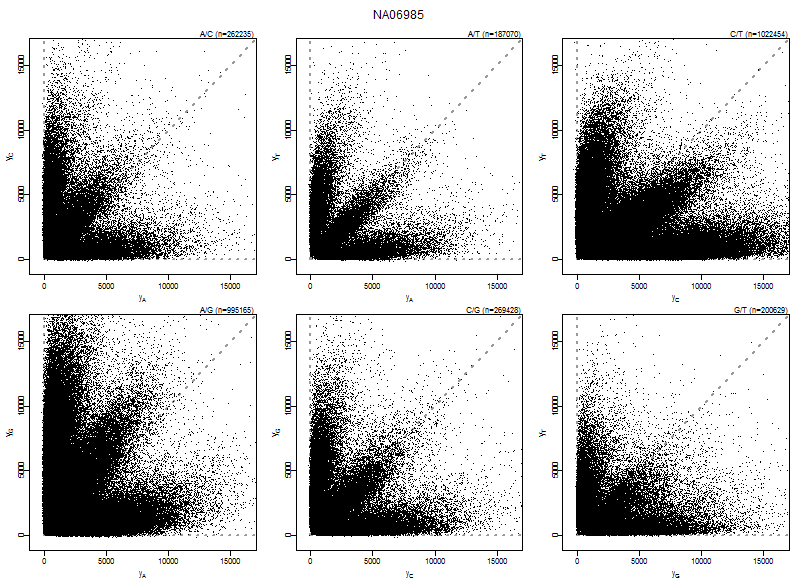
Figure: Allele probe pair intensities (PMA,PMB) of array NA06985 for the six nucleotide pairs (A,C), (A,G), (A,T), (C,G), (C,T), and (G,T). Data shown is before calibration.
plotAllelePairs(acc, array=array, pairs=1:6, what="output", xlim=xlim)
 * *
* *
Figure: Allele probe pair intensities (PMA,PMB) of array NA06985 for the six nucleotide pairs (A,C), (A,G), (A,T), (C,G), (C,T), and (G,T). Data shown is after calibration.
Step 2 - Normalization for nucleotide-position probe sequence effects
By using argument target="zero", no reference is required. Otherwise,
the average file will be used as the reference.
bpn <- BasePositionNormalization(csC, target="zero")
print(bpn)

BasePositionNormalization:
Data set: HapMap270
Input tags: 6.0,CEU,testSet,ACC,ra,-XY
User tags: *
Asterisk ('*') tags: BPN,-XY
Output tags: 6.0,CEU,testSet,ACC,ra,-XY,BPN,-XY
Number of files: 6 (394.42MB)
Platform: Affymetrix
Chip type: GenomeWideSNP_6,Full
Algorithm parameters: (unitsToFit: chr "-XY", typesToFit: chr "pm",
unitsToUpdate: NULL, typesToUpdate: chr "pm", shift: num 0, target: chr
"zero", model: chr "smooth.spline", df: int 5)
Output path:
probeData/HapMap270,6.0,CEU,testSet,ACC,ra,-XY,BPN,-XY/GenomeWideSNP_6
Is done: FALSE
RAM: 0.00MB
csN <- process(bpn, verbose=verbose)
print(csN)

AffymetrixCelSet:
Name: HapMap270
Tags: 6.0,CEU,testSet,ACC,ra,-XY,BPN,-XY
Path:
probeData/HapMap270,6.0,CEU,testSet,ACC,ra,-XY,BPN,-XY/GenomeWideSNP_6
Platform: Affymetrix
Chip type: GenomeWideSNP_6,Full
Number of arrays: 6
Names: NA06985, NA06991, ..., NA07019
Time period: 2008-11-28 16:03:45 -- 2008-11-28 16:36:42
Total file size: 394.42MB
RAM: 0.01MB
Benchmarking: Depending on system, this takes approximately 2-8min/array.
cs <- csN
par(mar=c(4,4,1,1)+0.1)
plotDensity(cs, lwd=2, ylim=c(0,0.40))
stext(side=3, pos=0, getFullName(cs))

Figure: The empirical densities for each of the arrays in the data set after crosstalk calibration and nucleotide-position normalization.
array <- 1
xlim <- c(-500,15000)
acc2 <- AllelicCrosstalkCalibration(csN)
plotAllelePairs(acc2, array=array, pairs=1:6, what="input", xlim=1.5*xlim)

Figure: Allele probe pair intensities (PMA,PMB) of array NA06985 for the six nucleotide pairs (A,C), (A,G), (A,T), (C,G), (C,T), and (G,T). Data shown is after crosstalk calibration and nucleotide-position normalization. Note how the heterozygote arms are along the diagonals, that is, there is a balance in the allele A and allele B signal for heterozygotes. This is (on purpose) not corrected for in the allelic crosstalk calibration.
Step 3 - Probe summarization
Next we summarize the probe level data unit by unit. For SNPs we have
the option to model either the total CN signals (combineAlleles=TRUE) or
allele-specific signals (combineAlleles=FALSE). Here we fit total CN
signals.
plm <- AvgCnPlm(csN, mergeStrands=TRUE, combineAlleles=TRUE)
print(plm)

AvgCnPlm:
Data set: HapMap270
Chip type: GenomeWideSNP_6,Full
Input tags: 6.0,CEU,testSet,ACC,ra,-XY,BPN,-XY
Output tags: 6.0,CEU,testSet,ACC,ra,-XY,BPN,-XY,AVG,A+B
Parameters: (probeModel: chr "pm"; shift: num 0; flavor: chr "median"
mergeStrands: logi TRUE; combineAlleles: logi TRUE).
Path:
plmData/HapMap270,6.0,CEU,testSet,ACC,ra,-XY,BPN,-XY,AVG,A+B/GenomeWideSNP_6
RAM: 0.00MB
Comment on the probe-summarization model:
AvgCnPlm summarizes probes by taking the robust average without
modeling probe affinities. This makes sense for the GenomeWideSNP_5
and GenomeWideSNP_6 chip types where all replicated probes in a probe
set are identical technical replicates which we expect to have the same
probe affinities. Since all probe affinities are the same, the
probe-affinity terms vanish if we consider multi-array models such as
the log-additive one of RmaCnPlm. For earlier chip types (10K-500K) it
still make sense to use the RmaCnPlm class. To use the latter, just
replace AvgCnPlm with RmaCnPlm above.
if (length(findUnitsTodo(plm)) > 0) {
  # Fit CN probes quickly (~5-10s/array + some overhead)
  units <- fitCnProbes(plm, verbose=verbose)
  str(units)
  # int [1:945826] 935590 935591 935592 935593 935594 935595 ...

  # Fit remaining units, i.e. SNPs (~5-10min/array)
  units <- fit(plm, verbose=verbose)
  str(units)
}

ces <- getChipEffectSet(plm)
print(ces)

CnChipEffectSet:
Name: HapMap270
Tags: 6.0,CEU,testSet,ACC,ra,-XY,BPN,-XY,AVG,A+B
Path:
plmData/HapMap270,6.0,CEU,testSet,ACC,ra,-XY,BPN,-XY,AVG,A+B/GenomeWideSNP_6
Platform: Affymetrix
Chip type: GenomeWideSNP_6,Full,monocell
Number of arrays: 6
Names: NA06985, NA06991, ..., NA07019
Time period: 2008-11-29 21:46:31 -- 2008-11-29 21:46:32
Total file size: 161.70MB
RAM: 0.01MB
Parameters: (probeModel: chr "pm", mergeStrands: logi TRUE,
combineAlleles: logi TRUE)
Step 4 - Normalization for PCR fragment-length effects
Similarly to how we normalized for the probe-sequence effects, we will
here normalize for PCR fragment-length effects by using a "zero"
target. This will avoid using the average (chip effects) as a
reference. Thus, this step is also truly single-array by nature.
fln <- FragmentLengthNormalization(ces, target="zero")
print(fln)

FragmentLengthNormalization:
Data set: HapMap270
Input tags: 6.0,CEU,testSet,ACC,ra,-XY,BPN,-XY,AVG,A+B
User tags: *
Asterisk ('*') tags: FLN,-XY
Output tags: 6.0,CEU,testSet,ACC,ra,-XY,BPN,-XY,AVG,A+B,FLN,-XY
Number of files: 6 (161.70MB)
Platform: Affymetrix
Chip type: GenomeWideSNP_6,Full,monocell
Algorithm parameters: (subsetToFit: chr "-XY", onMissing: chr "median",
.target: chr "zero", shift: num 0)
Output path:
plmData/HapMap270,6.0,CEU,testSet,ACC,ra,-XY,BPN,-XY,AVG,A+B,FLN,-XY/GenomeWideSNP_6
Is done: FALSE
RAM: 0.00MB
cesN <- process(fln, verbose=verbose)
print(cesN)

CnChipEffectSet:
Name: HapMap270
Tags: 6.0,CEU,testSet,ACC,ra,-XY,BPN,-XY,AVG,A+B,FLN,-XY
Path:
plmData/HapMap270,6.0,CEU,testSet,ACC,ra,-XY,BPN,-XY,AVG,A+B,FLN,-XY/GenomeWideSNP_6
Platform: Affymetrix
Chip type: GenomeWideSNP_6,Full,monocell
Number of arrays: 6
Names: NA06985, NA06991, ..., NA07019
Time period: 2008-11-29 21:46:31 -- 2008-11-29 21:46:32
Total file size: 161.70MB
RAM: 0.01MB
Parameters: (probeModel: chr "pm", mergeStrands: logi TRUE,
combineAlleles: logi TRUE)
Step 5 - Calculation of raw copy numbers
The above cesN object contains chip-effect estimates according to the
CRMA v2 method (Bengtsson, Wirapati, and Speed, 2009). In this
section we will show how to calculate raw copy numbers relative to a
reference. Note that several of the downstream methods, such as
segmentation methods, will do this automatically/internally and
therefore it is often not necessary to do this manually.
Deciding on a reference
There are two common use cases for CN analysis; either one do (i) a paired analysis where each sample is coupled with a unique reference (e.g. tumor/normal) or (ii) a non-paired analysis where each sample use the same common reference. When a common reference is used, it is often the average of a pool of samples. Here we will show how to do the latter.
Calculating the robust average of all samples
To calculate the robust average of chip effects across all existing samples (i=1,2,...,I), that is,
theta_Rj = median_i {theta_ij}
for each unit j=1,2,...,J. This calculation can be done as:
ceR <- getAverageFile(cesN, verbose=verbose)
print(ceR)

CnChipEffectFile:
Name: .average-intensities-median-mad
Tags: 036dedb6629c761a032d97b5c23bc278
Pathname:
plmData/HapMap270,6.0,CEU,testSet,ACC,ra,-XY,BPN,-XY,AVG,A+B,FLN,-XY/GenomeWideSNP_6/.average-intensities-median-mad,036dedb6629c761a032d97b5c23bc278.CEL
File size: 26.95MB
RAM: 0.01MB
File format: v4 (binary; XDA)
Platform: Affymetrix
Chip type: GenomeWideSNP_6,Full,monocell
Timestamp: 2008-12-09 14:40:43
Parameters: (probeModel: chr "pm", mergeStrands: logi TRUE,
combineAlleles: logi TRUE)
From the output we learn that ceR is a CnChipEffectFile just like the
other arrays in the cesN set. From now on we can treat it as if it
was the output a hybridization although it is actually the average over
many. The main difference is that this one is likely to have more
precise chip effects (because of the averaging over many estimates).
Extracting chip-effect estimates
The next step is to calculate the relative copy numbers:
C_ij = 2*theta_ij / theta_Rj
where we assume the copy-neutral state has two (2) copies. In order to calculate this, we need to extract theta_ij and theta_Rj.
Example: A single unit in one sample
Consider array i=3 and unit j=987. We can then extract these values as:
ce <- cesN[[3]]  # Array #3
theta <- extractTheta(ce, unit=987)
thetaR <- extractTheta(ceR, unit=987)
C <- 2*theta/thetaR
print(C)
          [,1]
[1,] 1.917
Thus, for array #3 (NA06993) and unit #987 (SNP_A-4268099), the estimated total raw copy number is C=1.92. If the DNA extract is homogeneous (containing only the same normal cells), we expect this to correspond to a truly diploid locus.
If we look at the individual theta and thetaR estimates,
print(c(theta, thetaR))
 [1] 2570 2681
we find that, on average (robust), an array has chip-effect signal 2681 (on the intensity scale). This is the signal we expect a copy neutral event at this particular locus to have.
Example: A small region on chromosome 2 in one sample
Next we are interested in the distribution of raw copy number {C_ij} in a small region on chromosome 2 in sample NA06991.
# Identification of units in Chr 2:81-86MB and their positions
cdf <- getCdf(cesN)
gi <- getGenomeInformation(cdf)
units <- getUnitsOnChromosome(gi, chromosome=2, region=c(81,86)*1e6)
pos <- getPositions(gi, units=units)

# Retrieving CN estimates of the reference in the above region
ceR <- getAverageFile(cesN)
thetaR <- extractTheta(ceR, units=units)

# Retrieving the corresponding estimates of sample NA06985
ce <- cesN[[indexOf(cesN, "NA06985")]]
theta <- extractTheta(ce, units=units)

# Calculate the relative CNs
C <- 2*theta/thetaR

# Plotting data along genome par(mar=c(3,4,2,1)+0.1)
plot(pos/1e6, C, pch=".", cex=3, ylim=c(0,4))
stext(side=3, pos=0, getName(ce))
stext(side=3, pos=1, "Chr2")

Figure: Copy number estimates in a 5.0Mb region on Chr2 for sample NA06985. There is a clear deletion at 83.1-83.7Mb.
Conclusions
We have shown how to estimate full-resolution ("raw") total copy numbers using the CRMA v2 method presented in (Bengtsson, Wirapati, and Speed, 2009). These estimates can be used for various purposes, where segmentation for identifying CN regions is the most common one. For details on how to apply downstream methods, see other aroma.affymetrix vignettes.
See also
-
doCRMAv2()- a convenient wrapper that runs CRMA v2 in one call.
References
[1] H. Bengtsson, R. Irizarry, B. Carvalho, et al. "Estimation and assessment of raw copy numbers at the single locus level". Eng. In: Bioinformatics (Oxford, England) 24.6 (Mar. 2008), pp. 759-67. ISSN: 1367-4811. DOI: 10.1093/bioinformatics/btn016. PMID: 18204055.
[2] H. Bengtsson, P. Wirapati, and T. P. Speed. "A single-array preprocessing method for estimating full-resolution raw copy numbers from all Affymetrix genotyping arrays including GenomeWideSNP 5 & 6". Eng. In: Bioinformatics (Oxford, England) 25.17 (Sep. 2009), pp. 2149-56. ISSN: 1367-4811. DOI: 10.1093/bioinformatics/btp371. PMID: 19535535.