Vignette: CRLMM genotyping (100K and 500K)
Author: Henrik Bengtsson
Created on: 2009-01-15
Last updated: 2009-01-15
Introduction
This document shows how to estimate genotypes based on the CRLMM
algorithm (Carvalho, Bengtsson, Speed, and Irizarry, 2007). The setup is such that it tries to replicate the estimates
of the justCRLMMv2() of the oligo package. Support for CRLMM in
aroma.affymetrix is currently for the 100K and the 500K chip types. The
GWS5 or GWS6 chip types are yet not supported.
Setup
If this is your first analysis in aroma.affymetrix, please make sure to first read the first few pages in the online 'Users Guide'. This will explain the importance of following a well defined directory structure and file names. Understanding this is important and will save you a lot of time.
Annotation data
annotationData/
    chipTypes/
      Mapping250K_Nsp/
       Mapping250K_Nsp.cdf
       Mapping250K_Nsp,na26,HB20080915.ugp
Raw data
rawData/
   HapMap270,500K,CEU,testSet/
     Mapping250K_Nsp/
       NA06985.CEL    NA06991.CEL    NA06993.CEL
       NA06994.CEL    NA07000.CEL    NA07019.CEL
TThere should be 6 CEL files in total. This data was downloaded from the HapMap website.
Analysis
library("aroma.affymetrix")
log <- verbose <- Arguments$getVerbose(-8, timestamp=TRUE)
Setup raw data set
cdf <- AffymetrixCdfFile$byChipType("Mapping50K_Nsp")
print(cdf)

## AffymetrixCdfFile:
## Path: annotationData/chipTypes/Mapping250K_Nsp
## Filename: Mapping250K_Nsp.cdf
## Filesize: 185.45MB
## Chip type: Mapping250K_Nsp
## RAM: 11.01MB
## File format: v4 (binary; XDA)
## Number of cells: 6553600
## Number of units: 262338
## Cells per unit: 24.98
## Number of QC units: 6

csR <- AffymetrixCelSet$byName("HapMap270,500K,CEU,testSet", cdf=cdf)
print(csR)

## AffymetrixCelSet:
## Name: HapMap270
## Tags: 500K,CEU,testSet
## Path: rawData/HapMap270,500K,CEU,testSet/Mapping250K_Nsp
## Platform: Affymetrix
## Chip type: Mapping250K_Nsp
## Number of arrays: 6
## Names: NA06985, NA06991, ..., NA07019
## Time period: 2005-11-16 15:17:51 -- 2005-11-18 19:08:24
## Total file size: 375.88MB
## RAM: 0.01MB
SNPRMA (normalization and summarization)
ces <- justSNPRMA(csR, normalizeToHapmap=TRUE, returnESet=FALSE, verbose=log)
print(ces)

## SnpChipEffectSet:
## Name: HapMap270
## Tags: 500K,CEU,testSet,QN,HapMapRef,RMA,oligo,+-
## Path: plmData/HapMap270,500K,CEU,testSet,QN,HapMapRef,RMA,oligo,+-/Mapping250K_Nsp
## Platform: Affymetrix
## Chip type: Mapping250K_Nsp,monocell
## Number of arrays: 6
## Names: NA06985, NA06991, ..., NA07019
## Time period: 2009-01-10 17:34:45 -- 2009-01-10 17:34:46
## Total file size: 57.34MB
## RAM: 0.01MB
## Parameters: (probeModel: chr "pm", mergeStrands: logi FALSE)
Genotype calling using the CRLMM model
Setting up the model:
crlmm <- CrlmmModel(ces, tags="*,oligo")
print(crlmm)

## CrlmmModel:
## Data set: HapMap270
## Chip type: Mapping250K_Nsp,monocell
## Input tags: 500K,CEU,testSet,QN,HapMapRef,RMA,oligo,+-
## Output tags: 500K,CEU,testSet,QN,HapMapRef,RMA,oligo,+-,CRLMM,oligo
## Parameters: (balance: num 1.5; minLLRforCalls: num [1:3] 5 1 5
## recalibrate: logi FALSE;flavor: chr "v2").
## Path: crlmmData/HapMap270,500K,CEU,testSet,QN,HapMapRef,RMA,oligo,+-,CRLMM,oligo/Mapping250K_Nsp
## RAM: 0.00MB
Fitting the model:
units <- fit(crlmm, ram="oligo", verbose=log)
str(units)

## int [1:262264] 135666 261964 227992 3670 227993 159191 212754 24401 ...
Accessing individual genotype calls and confidence scores
Retrieving the genotype calls (without actually loading anything):
callSet <- getCallSet(crlmm)
print(callSet)

## AromaUnitGenotypeCallSet:
## Name: HapMap270
## Tags: 500K,CEU,testSet,QN,HapMapRef,RMA,oligo,+-,CRLMM,oligo
## Full name: HapMap270,500K,CEU,testSet,QN,HapMapRef,RMA,oligo,+-,CRLMM,oligo
## Number of files: 6
## Names: NA06985, NA06991, ..., NA07019
## Path (to the first file): crlmmData/HapMap270,500K,CEU,testSet,QN,HapMapRef,RMA,oligo,+-,CRLMM,oligo/Mapping250K_Nsp
## Total file size: 3.00MB
## RAM: 0.01MB

calls <- extractGenotypes(callSet, units=2001:2005)
print(calls)

## NA06985 NA06991 NA06993 NA06994 NA07000 NA07019
## [1,] "AA" "AA" "AA" "AA" "AA" "AA"
## [2,] "AA" "AB" "AB" "BB" "AB" "AB"
## [3,] "AA" "AB" "AB" "AB" "AA" "AB"
## [4,] "BB" "AB" "AB" "BB" "BB" "BB"
## [5,] "AA" "AA" "AA" "AA" "AA" "AA"
Retrieving the confidence scores for the calls:
confSet <- getConfidenceScoreSet(crlmm)
print(confSet)

## AromaUnitSignalBinarySet:
## Name: HapMap270
## Tags: 500K,CEU,testSet,QN,HapMapRef,RMA,oligo,+-,CRLMM,oligo
## Full name: HapMap270,500K,CEU,testSet,QN,HapMapRef,RMA,oligo,+-,CRLMM,oligo
## Number of files: 6
## Names: NA06985, NA06991, ..., NA07019
## Path (to the first file): crlmmData/HapMap270,500K,CEU,testSet,QN,HapMapRef,RMA,oligo,+-,CRLMM,oligo/Mapping250K_Nsp
## Total file size: 6.01MB
## RAM: 0.01MB

scores <- extractMatrix(confSet, units=2001:2005)
print(scores)

## NA06985 NA06991 NA06993 NA06994 NA07000 NA07019
## [1,] 0.9998 0.9998 0.9998 0.9999 0.9999 0.9998
## [2,] 0.9968 0.9932 0.9931 0.9998 0.9976 0.9974
## [3,] 0.9997 0.9993 0.9967 0.9988 0.9998 0.9975
## [4,] 0.9986 0.9961 0.9894 0.9994 0.9994 0.9989
## [5,] 0.9998 0.9999 0.9998 0.9999 0.9998 0.9998
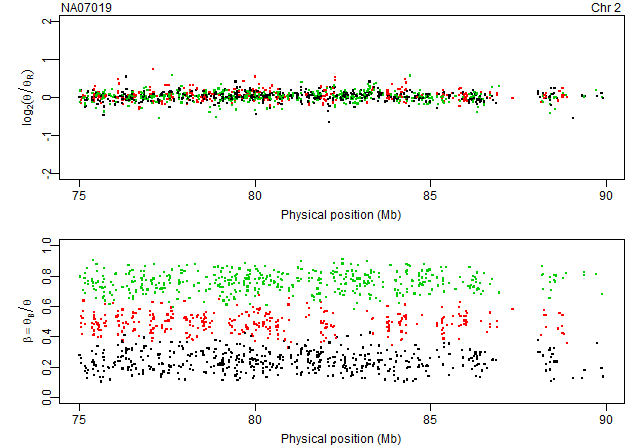
Plotting raw CNs and raw genotypes annotated by genotypes
gi <- getGenomeInformation(cdf)
units <- getUnitsOnChromosome(gi, chromosome=2, region=c(75,90)*1e6)
pos <- getPositions(gi, units=units) / 1e6
Get data for the last array:
array <- 6
ce <- ces[[array]]
data <- extractTotalAndFreqB(ce, units=units)
str(data)

## num [1:1306, 1:2] 2312 2185 1994 3242 4156 ...
## - attr(*, "dimnames")=List of 2
## ..$ : NULL
## ..$ : chr [1:2] "total" "freqB"
Extract the (total) theta and the freqB columns:
theta <- data[,"total"]
freqB <- data[,"freqB"]
We calculate the copy-neutral reference as the robust average of all arrays:
ceR <- getAverageFile(ces)
dataR <- extractTotalAndFreqB(ceR, units=units)
thetaR <- dataR[,"total"]
Then we calculate the log2 copy-number ratios:
M <- log2(theta/thetaR)
Finally, we extract the corresponding genotype calls:
cf <- callSet[[array]]
calls <- extractGenotypes(cf, units=units)
Next, we plot the (x,C) and (x,freqB) along the genome annotated with colors according to genotype:
col <- c(AA=1, AB=2, BB=3)[calls]
xlim <- range(pos, na.rm=TRUE)
xlab <- "Physical position (Mb)"
Mlab <- expression(log[2](theta/theta[R]))
Blab <- expression(beta == theta[B]/theta)
subplots(2, ncol=1)
par(mar=c(3,4,1,1)+0.1, pch=".")
plot(pos, M, col=col, cex=3, xlim=xlim, ylim=c(-2,2), xlab=xlab, ylab=Mlab)
stext(side=3, pos=0, getName(ce))
stext(side=3, pos=1, "Chr 2")
plot(pos, freqB, col=col, cex=3, xlim=xlim, ylim=c(0,1), xlab=xlab, ylab=Blab)
Comparing with CRLMM in oligo
path <- file.path("oligoData", getFullName(csR), getChipType(csR, fullname=FALSE))
path <- Arguments$getWritablePathname(path)
if (!isDirectory(path)) {
  mkdirs(getParent(path))
  oligo:::justCRLMMv2(getPathnames(csR), tmpdir=path, recalibrate=FALSE, balance=1.5, verbose=TRUE)
}
Comparing genotype calls
Genotype calls according to oligo
calls0 <- readSummaries("calls", path)
dimnames(calls0) <- NULL
Genotype calls according to aroma.affymetrix
units <- indexOf(cdf, pattern="^SNP")
unitNames <- getUnitNames(cdf, units=units)
units <- units[order(unitNames)]
calls <- extractGenotypes(callSet, units=units, encoding="oligo")
dimnames(calls) <- NULL
Differences between aroma.affymetrix and oligo
count <- 0
for (cc in 1:ncol(calls)) {
  idxs <- which(calls[,cc] != calls0[,cc])
  count <- count + length(idxs)
  printf("%s: ", getNames(callSet)[cc])
  if (length(idxs) > 0) {
    map <- c("AA", "AB", "BB")
    cat(paste(map[calls[idxs,cc]], map[calls0[idxs,cc]], sep="!="), sep=",")
  }
  cat("\n")
}
We identify the following difference for each of the genotyped samples:
- NA06985: AB!=AA, AB!=BB, AB!=AA, BB!=AB, BB!=AB
- NA06991: AB!=AA
- NA06993: AA!=AB, BB!=AB
- NA06994: AB!=AA, BB!=AB
- NA07000: AB!=BB, AA!=AB
- NA07019: AA!=AB, AA!=AB, AA!=AB, AA!=AB
Note that these differences are only in one allele, that is, one implementation calls a SNP heterozygote whereas the other calls a homozygote.
printf("Averages number of discrepancies per array: %.1f\n", count/ncol(calls))
Averages number of discrepancies per array: 2.7
errorRate <- count/length(calls)
printf("Concordance rate: %.5f%%\n", 100*(1-errorRate))
Concordance rate: 99.99898%
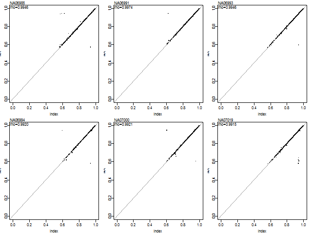
Comparing confidence scores
Confidence scores according to oligo:
conf0 <- readSummaries("conf", path)
dimnames(conf) <- NULL
Confidence scores according to aroma.affymetrix:
conf <- extractMatrix(confSet, units=units)
dimnames(conf) <- NULL
Differences between aroma.affymetrix and oligo:
delta <- conf - conf0
avgDelta <- mean(abs(delta), na.rm=TRUE)
printf("Averages difference: %.2g\n", avgDelta)
Averages difference: 7.1e-06
Pairwise plots:
subplots(ncol(conf))
par(mar=c(3,2,1,1)+0.1)
lim <- c(0,1)
for (cc in 1:ncol(conf)) {
  plot(NA, xlim=lim, ylim=lim)
  abline(a=0, b=1, col="#999999")
  points(conf[,cc], conf0[,cc], pch=".", cex=3)
  rho <- cor(conf[,cc], conf0[,cc])
  stext(side=3, pos=0, line=-1, sprintf("rho=%.4f", rho))
  stext(side=3, pos=0, getNames(confSet)[cc])
  printf("Array #%d: Correlation: %.4f\n", cc, rho)
}
References
[1] B. Carvalho, H. Bengtsson, T. P. Speed, et al. "Exploration, normalization, and genotype calls of high-density oligonucleotide SNP array data". Eng. In: Biostatistics (Oxford, England) 8.2 (Apr. 2007), pp. 485-99. ISSN: 1465-4644. DOI: 10.1093/biostatistics/kxl042. PMID: 17189563.
Appendix
Session information
> sessionInfo()

R version 2.8.1 Patched (2008-12-22 r47296)
 i386-pc-mingw32
 locale:
 LC_COLLATE=English_United States.1252;LC_CTYPE=English_United
States.1252;LC_MONETARY=English_United
States.1252;LC_NUMERIC=C;LC_TIME=English_United States.1252

attached base packages:

[1] splines tools stats graphics grDevices utils datasets
[8] methods base

other attached packages:

[1] pd.mapping250k.nsp_0.4.1 oligoClasses_1.3.8
[4] AnnotationDbi_1.3.12 preprocessCore_1.3.4 RSQLite_0.7-0
[7] DBI_0.2-4 Biobase_2.1.7 aroma.affymetrix_1.0.0
[10] aroma.apd_0.1.4 R.huge_0.1.6 affxparser_1.15.1
[13] aroma.core_1.0.0 aroma.light_1.11.1 oligo_1.5.9
[16] digest_0.3.1 matrixStats_0.1.3 R.rsp_0.3.4
[19] R.cache_0.1.7 R.utils_1.1.3 R.oo_1.4.6
[22] R.methodsS3_1.0.3