Vignette: Total Copy Number Analysis (GWS5 & GWS6)

Author: Henrik Bengtsson
Created: 2007-11-25
Last updated: 2009-01-26

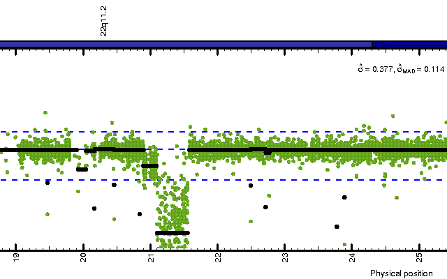
Figure: A region on Chr22 in HapMap sample NA06994 showing two deletions each with different copy number means.

This document will explain how to do total copy-number analysis on GenomeWideSNP_6 (aka "6.0", "SNP6" and "GWS6") data. Although we will use 6.0 data in the example, the exact same code can be used for GenomeWideSNP_5 (aka "5.0", "SNP5" and "GWS5") data. The only difference is what annotation files are used.

We will go through how to setup the data set, calibrate it for allelic crosstalk, then summarize the probe data in order to obtain so called chip effects, which we then normalize for PCR fragment-length effects as well as for imbalances in NspI and StyI mixes. The normalize chip effects are then passed to the Circular Binary Segmentation (CBS) methods, which identifies aberrant regions in the genome. The results will be browsable in the ChromosomeExplorer (see Figure above).

A small disclaimer: The outlined method is not final and is under development. Especially note that we no longer have a multichip probe-level model that protects us against outliers. Instead such outliers has to be dealt with by the segmentation method. However, we find it good enough at this stage in order for us to share it.

Setup

Raw data

• Test set: HapMap270,6.0,CEU,testSet
• Test samples: NA06985, NA06991, NA06993, NA06994, NA07000, NA07019
• Path: rawData/HapMap270,6.0,CEU,testSet/GenomeWideSNP_6/

Annotation data

GenomeWideSNP_6

Here we will work with GenomeWideSNP_6 data. Get the following annotation files and place them in annotationData/chipTypes/GenomeWideSNP_6/:

• GenomeWideSNP_6,Full.cdf: The "full" CDF from Affymetrix. Use the GenomeWideSNP_6.Full.cdf, but make sure to rename it by replacing the dots in the name with commas. To confirm that you have the 'full' CDF file, check the number of units, e.g with print(cdf). The full CDF file has 1881415 units.
• GenomeWideSNP_6,Full,na24,HB20080214.ugp: The Unit Genome Position (UGP) file.
• GenomeWideSNP_6,Full,na24,HB20080214.ufl: The Unit Fragment Length (UFL) file.

You will find the UGP and UFL files on Page GenomeWideSNP_6. There you will also more information about this chip type, and find links to the Affymetrix website where you can download the CDF.

GenomeWideSNP_5

If you work with GenomeWideSNP_5 data, get the following annotation files and place them in annotationData/chipTypes/GenomeWideSNP_5/:

• GenomeWideSNP_5,Full,r2.cdf: The "full" and "alternative" CDF from Affymetrix. Use the GenomeWideSNP_5.Full.r2.cdf, but make sure to rename it by replacing the dots in the name with commas.
• GenomeWideSNP_5,Full,r2,na24,HB20080302.ugp: The Unit Genome Position (UGP) file.
• GenomeWideSNP_5,Full,r2,na24,HB20080214.ufl: The Unit Fragment Length (UFL) file.

You will find the UGP and UFL files on Page GenomeWideSNP_5. There you will also more information about this chip type, and find links to the Affymetrix website where you can download the CDF. It is important that you get the "alternative CDF", which is indicated with 'r2' (revision 2), not the original CDF.

Low-level analysis

library("aroma.affymetrix")
verbose <- Arguments$getVerbose(-8, timestamp=TRUE)

Verifying annotation data files

Affymetrix provides two different CDF files for the GenomeWideSNP_6 chip type, namely the "default" and "full" CDF. The full CDF contains what the default one does plus more. We are always using the full CDF. We start by locating this CDF:

cdf <- AffymetrixCdfFile$byChipType("GenomeWideSNP_6", tags="Full")
print(cdf)

gives

AffymetrixCdfFile:
Path: annotationData/chipTypes/GenomeWideSNP_6
Filename: GenomeWideSNP_6,Full.CDF
Filesize: 470.44MB
File format: v4 (binary; XDA)
Chip type: GenomeWideSNP_6,Full
Dimension: 2572x2680
Number of cells: 6892960
Number of units: 1881415
Cells per unit: 3.66
Number of QC units: 4
RAM: 0.00MB

Before we continue, the following will assert that the UFL and the UGP annotation files can be found and that they are compatible with the give CDF. These step are not really needed for analysis, because they are done in the background, but it is a good test to see that the setup is correct and catch any errors in setup already here.

gi <- getGenomeInformation(cdf)
print(gi)

gives:

UgpGenomeInformation:
Name: GenomeWideSNP_6
Tags: Full,na24,HB20080214
Pathname: annotationData/chipTypes/GenomeWideSNP_6/GenomeWideSNP_6,Full,na24,HB20080214.ugp
File size: 8.97MB
RAM: 0.00MB
Chip type: GenomeWideSNP_6,Full

si <- getSnpInformation(cdf)
print(si)

gives:

UflSnpInformation:
Name: GenomeWideSNP_6
Tags: Full,na24,HB20080214
Pathname: annotationData/chipTypes/GenomeWideSNP_6/GenomeWideSNP_6,Full,na24,HB20080214.ufl
File size: 7.18MB
RAM: 0.00MB
Chip type: GenomeWideSNP_6,Full
Number of enzymes: 2

Defining CEL set

The following will setup the CEL set using the full CDF specified above:

cs <- AffymetrixCelSet$byName("HapMap270,6.0,CEU,testSet", cdf=cdf)
print(cs)

gives:

AffymetrixCelSet:
Name: HapMap270
Tags: 6.0,CEU,testSet
Path: rawData/HapMap270,6.0,CEU,testSet/GenomeWideSNP_6
Chip type: GenomeWideSNP_6,Full
Number of arrays: 6
Names: NA06985, NA06991, ..., NA07019
Time period: NA -- NA
Total file size: 395.13MB
RAM: 0.01MB

Note how the chip type of the CEL set indicates that the full CDF is in use.

Calibration for allelic crosstalk

The first thing we will do is calibrate the probe signals such that offset in and crosstalk between alleles in the SNPs is removed. Offset is also removed from the CN probes. Finally, the probe signals are rescaled such that all probes not on ChrX and ChrY all have the same average for all arrays (=2200). Allelic crosstalk calibration is a single-array method, that is, each array is calibrated independently of the others. This means that you can use this method to calibrate a single array and having more arrays will not make different.

acc <- AllelicCrosstalkCalibration(cs)
print(acc)

gives:

AllelicCrosstalkCalibration:  
Data set: HapMap270  
Input tags: 6.0,CEU,testSet  
Output tags: 6.0,CEU,testSet,ACC,ra,-XY  
Number of arrays: 6 (395.13MB)  
Chip type: GenomeWideSNP_6,Full  
Algorithm parameters: (rescaleBy: chr "all", targetAvg: num 2200,
subsetToAvg: chr "-XY", alpha: num [1:5] 0.1 0.075 0.05 0.03 0.01, q:
num 2, Q: num 98)  
Output path:
probeData/HapMap270,6.0,CEU,testSet,ACC,ra,-XY/GenomeWideSNP_6  
Is done: FALSE
RAM: 0.00MB

First of all, it is important to understand that the above code does not calibrate the data set, but instead it sets up the method for doing so. We will do that in the next step. But first note how tags 'ACC,ra,-XY' are appended to the data set name. The 'ACC' tag indicates Allelic-Crosstalk Calibration, the 'ra' tags indicates that afterward all values are rescaled together ("rescale all"), and the tag '-XY' indicates that units on ChrX & ChrY are excluded from the model fit (estimate of the calibration parameters). This is the default behavior and is done in order to avoid XX and XY samples being artificially shrunk toward each other. However, note that all units are still calibrated.

To calibrate the probe signals, do:

csC <- process(acc, verbose=verbose)
print(csC)

which after a while will give:

AffymetrixCelSet:
Name: HapMap270
Tags: 6.0,CEU,testSet,ACC,ra,-XY
Path: probeData/HapMap270,6.0,CEU,testSet,ACC,ra,-XY/GenomeWideSNP_6
Chip type: GenomeWideSNP_6,Full
Number of arrays: 6
Names: NA06985, NA06991, ..., NA07019
Time period: 2007-12-09 02:32:49 -- 2007-12-09 02:54:05
Total file size: 394.42MB
RAM: 0.01MB

This takes approximately 1.5-2 mins per array.

Comment: If you are processing 6.0 arrays, it is likely that the original CEL files are in the new AGCC/Calvin file format. Since aroma.affymetrix can currently only read such files but not write them, the calibrated/normalized data is stored as binary/XDA CEL file. Because of this "conversion", the creation of the CEL files will take some time. Downstream analysis will then all be done using binary/XDA CEL files, and the above slowdown will not be observed.

Summarization

For the SNP & CN chip types all probes are technical replicates, why it makes little sense to model probe affinities (because all probes within a probeset should have identical affinities). Without probe affinities, the model basically becomes a single-array model. Thus, probe-level summarization for these newer chip types is effectively done for each array independently (although the implementation processing the data in multi-chip fashion). For total copy number analysis ignoring strand information, probe signals for SNPs are averaged across replicates and summarized between alleles, and probe signals for CN probes, which are all single-probe units, are left as it. Since some probe signals might become negative (by chance) from the allelic crosstalk calibration and due to random errors around zero, we offset of probe signals 300 units. This model is set up as:

plm <- AvgCnPlm(csC, mergeStrands=TRUE, combineAlleles=TRUE, shift=+300)
print(plm)

gives:

AvgCnPlm:
Data set: HapMap270
Chip type: GenomeWideSNP_6,Full
Input tags: 6.0,CEU,testSet,ACC,ra,-XY
Output tags: 6.0,CEU,testSet,ACC,ra,-XY,AVG,+300,A+B
Parameters: (probeModel: chr "pm"; shift: num 300; flavor: chr "median"
mergeStrands: logi TRUE; combineAlleles: logi TRUE).
Path:
plmData/HapMap270,6.0,CEU,testSet,ACC,ra,-XY,AVG,+300,A+B/GenomeWideSNP_6
RAM: 0.00MB

Note how tags 'AVG,+300,A+B' are added. The first one indicates that an AvgPlm was used, '+300' that the input data was shifted (translated) +300 before being fitted, and 'A+B' indicates that allele A and allele B probe pairs are summed together before being fitted, i.e. PM=PM_A+PM_B, since combineAlleles=TRUE.

By the way, all the SNPs in the GWS6 chip type only holds probes from one of the two strands, which means that the argument mergeStrands has no effect but it adds a tag indicating what value was used. The same holds for GWS5.

As with cross-talk calibration, no data is yet processed. In order fit the PLM defined above, we call:

if (length(findUnitsTodo(plm)) > 0) {
    # Fit CN probes quickly (\~5-10s/array + some overhead)
   units <- fitCnProbes(plm, verbose=verbose)
   str(units)
   # int [1:945826] 935590 935591 935592 935593 935594 935595 ...

  # Fit remaining units, i.e. SNPs (\~5-10min/array)
   units <- fit(plm, verbose=verbose)
   str(units)
}

This will take some time! Moreover, if it is the first time you process a given chip type, then a so called "monocell" CDF needs to be created, which in turn takes quite some time. When you later process data for the same chip type, the monocell CDF is already available (it is saved in the annotationData/chipTypes/GenomeWideSNP_6/ directory).

A note on non-positive signals and NaN estimates: Whenever calibrating for allelic crosstalk, one obtains some non-positive signals. Indeed, with 50% homozygote (AA and BB) SNPs, and if you assume symmetric noise, then actually half of the calibrated homozygote probe signals will be below zero and half above zero, i.e. for genotype AA there are 50% negative allele B signals and vice versa for genotype BB. Thus, 25% of your probe allele signals for SNPs may be non-positive if the crosstalk calibration is "perfect". For total copy number analysis we can add the allele A and allele B signals such that we partly avoid this problem. However, there will still be some signals there are zero or negative although they are summed. When fitting the log additive model, these values will become NaN when taking the logarithm, which is why you will see warnings on:

"In log(y, base=2) : NaNs produced"

These warnings are expected. Such data points will be ignored (fitted with zero weight) when fitting the log-additive model for probe sets. However, by chance some probesets will have all missing values because of this and therefore the estimated chip effects will also be NaN. To lower the risk for this we can add some offset back, which is what the shift=+300 does. For a further discussion on non-positive values, see Bengtsson, Irizarry, Carvalho, and Speed (2008).

When fitting a probe-level model, one set of estimates are the chip effects, which we later will use to estimate raw copy numbers. You can get the chip-effect set and see where they are stored etc. by calling:

ces <- getChipEffectSet(plm)
print(ces)

## CnChipEffectSet:
## Name: HapMap270
## Tags: 6.0,CEU,testSet,ACC,ra,-XY,AVG,+300,A+B
## Path: plmData/HapMap270,6.0,CEU,testSet,ACC,ra,-XY,AVG,+300,A+B/GenomeWideSNP_6
## Chip type: GenomeWideSNP_6,Full,monocell
## Number of arrays: 6
## Names: NA06985, NA06991, ..., NA07019
## Time period: 2007-12-09 02:56:57 -- 2007-12-09 02:57:00
## Total file size: 161.70MB
## RAM: 0.01MB
## Parameters: (probeModel: chr "pm", mergeStrands: logi TRUE,
## combineAlleles: logi TRUE)

Here we see that the chip type has now got the tag 'monocell' appended. This indicates that the chip-effect set is a special type of CEL set. The CEL files do not have the structure of the initial CDF (GenomeWideSNP_6,Full), but instead the structure of a monocell CDF, which is "miniature" of the initial CDF.

Final note, in the current implementation the CN probe units are treated as any other unit, although the probe summarization equals the probe intensity, which could be used to speed up the processing. We hope to improve the implementation in a future release resulting in a much faster processing of CN probes (basically instant).

PCR fragment length normalization

The probe-level summaries are currently structured and stored as if they were chip effects in a multi-chip PLM, which is why we still call them "chip effects". When preparing the target DNA, the DNA is digested and amplified in two parallel tracks using two different enzymes, namely NspI and StyI. This means that the units (SNPs and the CN probes) may be digested by either enzyme exclusively or both enzymes. The result are one or two fragments of different lengths per unit. When doing PCR, fragments of different lengths are amplified differently. Even more important, this systematic effect varies slightly from sample to sample. We have created a specific multi-chip model that controls for systematic effects across samples as a function of fragment lengths and enzyme mixtures. This model also controls for imbalances in NspI and StyI mixes. Details on the model will be published later.

Note that this normalization method is a multi-chip method. It estimate baseline (target) effects as the effects observed in a robust average across all arrays. Then each array is normalized such that it has the same effect as the baseline effect. Effectively, this approach will make systematic effects across arrays to cancel out. Having more arrays, will provide a more stable estimate of the baseline effect. Processing a single array will make no difference. Theoretically it should be possible to process as few as two arrays, but we have not studies of how well this works (overfitting etc).

To use the above model, do:

fln <- FragmentLengthNormalization(ces)
print(fln)

gives:

FragmentLengthNormalization:
Data set: HapMap270
Input tags: 6.0,CEU,testSet,ACC,ra,-XY,AVG,+300,A+B
Output tags: 6.0,CEU,testSet,ACC,ra,-XY,AVG,+300,A+B,FLN,-XY
Number of arrays: 6 (161.70MB)
Chip type: GenomeWideSNP_6,Full,monocell
Algorithm parameters: (subsetToFit: chr "-XY", .targetFunctions: NULL)
Output path:
plmData/HapMap270,6.0,CEU,testSet,ACC,ra,-XY,AVG,+300,A+B,FLN,-XY/GenomeWideSNP_6
Is done: FALSE
RAM: 0.00MB

Note how tags 'FLN,-XY' are added to indiciated that the output has been fragment-length normalized excluding ChrX & ChrY from the model fit. All units (that have fragment-length information) are still calibrated.

As before, the above is just a setup of a method. To actually normalize the chip effects, we do:

cesN <- process(fln, verbose=verbose)
print(cesN)

## CnChipEffectSet:
## Name: HapMap270
## Tags: 6.0,CEU,testSet,ACC,ra,-XY,AVG,+300,A+B,FLN,-XY
## Path: plmData/HapMap270,6.0,CEU,testSet,ACC,ra,-XY,AVG,+300,A+B,FLN,-XY/GenomeWideSNP_6
## Chip type: GenomeWideSNP_6,Full,monocell
## Number of arrays: 6
## Names: NA06985, NA06991, ..., NA07019
## Time period: 2007-12-09 02:56:57 -- 2007-12-09 02:57:00
## Total file size: 161.70MB
## RAM: 0.01MB
## Parameters: (probeModel: chr "pm", mergeStrands: logi TRUE, combineAlleles: logi TRUE)

Fragment-length normalization takes approximately 1 min/array.

Identification of copy-number regions (CNRs)

To run segmentation on raw CN estimates (log2 ratios) you can either use raw CNs calculated from case-control pairs of samples, or from samples relative to a common reference. In order to do paired analysis using the Circular Binary Segmentation (CBS) method, do:

cbs <- CbsModel(ces1, ces2)

where ces1 is a CEL set of test samples and ces2 is a CEL set of the same number of control samples. Use ces1 <- cesN[arrays1] and same for ces2 to extract the two sets from the cesN CEL set above.

Here we will focus on the non-paired case, where the common reference is
by default calculated as the robust average across samples.  To setup
the CBS model is this way, do:
```r
cbs <- CbsModel(cesN)
print(cbs)

gives:

CbsModel:
Name: HapMap270
Tags: 6.0,CEU,testSet,ACC,ra,-XY,AVG,+300,A+B,FLN,-XY
Chip type (virtual): GenomeWideSNP_6
Path:
cbsData/HapMap270,6.0,CEU,testSet,ACC,ra,-XY,AVG,+300,A+B,FLN,-XY/GenomeWideSNP_6
Number of chip types: 1
Chip-effect set & reference file pairs:
Chip type #1 of 1 ('GenomeWideSNP_6'):
Chip-effect set:
CnChipEffectSet:
Name: HapMap270
Tags: 6.0,CEU,testSet,ACC,ra,-XY,AVG,+300,A+B,FLN,-XY
Path: plmData/HapMap270,6.0,CEU,testSet,ACC,ra,-XY,AVG,+300,A+B,FLN,-XY/GenomeWideSNP_6
Chip type: GenomeWideSNP_6,Full,monocell
Number of arrays: 6
Names: NA06985, NA06991, ..., NA07019
Time period: 2007-12-09 02:56:57 -- 2007-12-09 02:57:00
Total file size: 161.70MB
RAM: 0.01MB
Parameters: (probeModel: chr "pm", mergeStrands: logi TRUE, combineAlleles: logi TRUE)
Reference file:
<average across arrays>
RAM: 0.00MB

The above tells us many things. First, we see that the output data is stored in a subdirectory of cbsData/. We see that there is only one chip type involved (for the 500K chip set, we would have two chip types merged in the segmentation). We see that the chip-effect set used is the one we got from fragment-length normalization. There is no reference set specified, so the reference for each sample defaults to the (robust) average across all samples.

Extracting raw copy numbers (optional)

This subsection is optional and may be skipped. Given any CopyNumberChromosomalModel, including GladModel, it is possible to extract raw copy numbers (log-ratios as defined in Bengtsson, Irizarry, Carvalho, et al. (2008) as follows:

rawCNs <- extractRawCopyNumbers(cbs, array=1, chromosome=1)
print(rawCNs)

## RawCopyNumbers:
## Number of loci: 40203
## Loci fields: cn [40203xnumeric], x [40203xnumeric]
## RAM: 0.61MB

This object holds (in memory) the raw CN estimates (cn) and their genomic locations (x) on the requested chromosome. The easiest way to work with this data is to turn it into a data frame:

rawCNs <- as.data.frame(rawCNs)
str(rawCNs)

## 'data.frame':   40203 obs. of  2 variables:
## $ x : num  742429 767376 769185 775852 782343 ...
## $ cn: num  -0.613 -0.715 -0.127 -0.349 -0.201 ...

Note that this can be done before/without fitting the copy-number model. Moreover, the raw CNs are estimates the exact same way regardless of CN model (GladModel, CbsModel, ...).

Fitting copy-number model and displaying results

We are next going to display the raw CNs and the segmentation results in the ChromosomeExplorer. As we will see, when asking the explorer to process a certain array and chromosome, it will in turn ask the segmentation model to fit that same data, if not already fitted. So, we take the following shortcut.

To fit CBS and at the same time generate graphical output for, say, chromosome 19, 22, and 23 (X), do:

ce <- ChromosomeExplorer(cbs)
print(ce)

which gives:

ChromosomeExplorer:
Name: HapMap270
Tags: 6.0,CEU,testSet,ACC,ra,-XY,AVG,+300,A+B,FLN,-XY
Number of arrays: 6
Path:
reports/HapMap270/6.0,CEU,testSet,ACC,ra,-XY,AVG,+300,A+B,FLN,-XY/GenomeWideSNP_6/cbs
RAM: 0.00MB

We see that the output will be stored under the reports/ directory. Note the slightly different layout of subdirectories compared with what we otherwise see. The first subdirectory is named after the data set without tags. Instead the tags alone specify the next level of subdirectory. This is done in order to collect reports for the same data set in the same directory tree.

To start fitting the segmentation model, generating plots and the explorer report, we do:

process(ce, chromosomes=c(19, 22, 23), verbose=verbose)

Note that, although CBS is currently the fastest segmentation available in aroma.affymetrix, these new chip type have so many markers per chromosome that the processing time will be substantial. The segmentation is currently what takes most of the time in CN analysis.

Finally, in order to view the ChromosomeExplorer, do:

display(ce)

which will launch your browser. You can also open the report manually by loading 'reports/HapMap270/6.0,CEU,testSet,ACC,ra,-XY,AVG,+300,A+B,FLN,-XY/ChromosomeExplorer.html' in the browser.

If for some reason we wanted to perform segmentation without displaying the results, we could have called:

fit(cbs, chromosomes=c(19, 22, 23), verbose=verbose)

to do segmentation on Chr19, Chr22 and ChrX. The estimated copy-number regions will be stored in files under cbsData/. If we then decide we wish to display the results, we can use the code above to do so (create ChromosomeExplorer object, process and display).

There may be cases in which only a subset of arrays is desired. In such instances we can use the arrays argument of process() or fit(), e.g.:

process(ce, arrays=1:2, chromosomes=c(19, 22, 23), verbose=verbose)
fit(cbs, arrays=1:2, chromosomes=c(19, 22, 23), verbose=verbose)

References

[1] H. Bengtsson, R. Irizarry, B. Carvalho, et al. "Estimation and assessment of raw copy numbers at the single locus level". Eng. In: Bioinformatics (Oxford, England) 24.6 (Mar. 2008), pp. 759-67. ISSN: 1367-4811. DOI: 10.1093/bioinformatics/btn016. PMID: 18204055.