Vignette: Empirical probe-signal densities and rank-based quantile normalization

Author: Henrik Bengtsson
Created on: 2009-09-17
Last updated: 2011-02-05

This document illustrated (i) how to create density plots of raw and normalized probe signals and (ii) the result of rank-based quantile normalization stratified by probe type.

Setup

Here we will use 10 public Mapping50K_Hind240 CEL files from the HapMap project.

Raw data

Download the following CEL files from the HapMap site (see the 'HapMap 100K' data set on Page Data Sets):

rawData/
  HapMap,CEU,testSet/
    Mapping50K_Hind240/
      NA06985_Hind_B5_3005533.CEL
      NA06991_Hind_B6_3005533.CEL
      NA06993_Hind_B4_4000092.CEL
      NA06994_Hind_A7_3005533.CEL
      NA07000_Hind_A8_3005533.CEL
      NA07019_Hind_A12_4000092.CEL
      NA07022_Hind_A10_4000092.CEL
      NA07029_Hind_A9_4000092.CEL
      NA07034_Hind_B1_4000092.CEL
      NA07048_Hind_B3_4000092.CEL

Annotation data

Download the following annotation files (Mapping50K_Hind240 & Mapping50K_Xba240):

annotationData/
  chipTypes/
    Mapping50K_Hind240/
      Mapping50K_Hind240.CDF
      Mapping50K_Hind240,na26,HB20080916.ufl
      Mapping50K_Hind240,na26,HB20080916.ugp

Startup

library("aroma.affymetrix")
library("R.devices")
devOptions("png", width=1024)

# Use a nicer palette of colors
colors <- RColorBrewer::brewer.pal(12, "Paired")
palette(colors)

# Setup the Verbose object
verbose <- Arguments$getVerbose(-10, timestamp=TRUE)

Setup of raw data set

cdf <- AffymetrixCdfFile$byChipType("Mapping50K_Hind240")
print(cdf)

gi <- getGenomeInformation(cdf)
print(gi)

Setup of raw data set

csR <- AffymetrixCelSet$byName("HapMap,CEU,testSet", cdf=cdf)
print(getFullNames(csR))

## [1] "NA06985_Hind_B5_3005533"  "NA06991_Hind_B6_3005533"
## [3] "NA06993_Hind_B4_4000092"  "NA06994_Hind_A7_3005533"
## [5] "NA07000_Hind_A8_3005533"  "NA07019_Hind_A12_4000092"
## [7] "NA07022_Hind_A10_4000092" "NA07029_Hind_A9_4000092"
## [9] "NA07034_Hind_B1_4000092"  "NA07048_Hind_B3_4000092"

The CEL files downloaded from HapMap has file names such as NA07000_Hind_A8_3005533.CEL. In order for aroma.affymetrix to identify 'NA07000' as the sample name, and 'A8' and '3005533' as tags (ignore the 'Hind' part), we will utilize so called fullname translators that translates the full name to a comma-separated fullname, e.g. 'NA07000_Hind_A8_3005533' to 'NA07000,A8,3005533'.

setFullNamesTranslator(csR, function(names, ...) {
  # Turn into comma-separated tags
  names <- gsub("_", ",", names)
  # Drop any Hind/Xba tags
  names <- gsub(",(Hind|Xba)", "", names)
  names
})
print(getFullNames(csR))

## [1] "NA06985,B5,3005533"  "NA06991,B6,3005533"
## [3] "NA06993,B4,4000092"  "NA06994,A7,3005533"
## [5] "NA07000,A8,3005533"  "NA07019,A12,4000092"
## [7] "NA07022,A10,4000092" "NA07029,A9,4000092"
## [9] "NA07034,B1,4000092"  "NA07048,B3,4000092"

print(csR)

## AffymetrixCelSet:
## Name: HapMap
## Tags: CEU,testSet
## Path: rawData/HapMap,CEU,testSet/Mapping50K_Hind240
## Platform: Affymetrix
## Chip type: Mapping50K_Hind240
## Number of arrays: 10
## Names: NA06985, NA06991, ..., NA07048
## Time period: 2004-01-14 14:02:08 -- 2004-02-13 11:51:01
## Total file size: 244.78MB
## RAM: 0.01MB

Brief about different types of probes

On Affymetrix arrays, there are different types of probes (cells). The most well known are perfect-match (PM) and mismatch (MM) probes. In addition to these, there are also QC probes, e.g. so called landing-light probes and chequered-flag probes etc.

One can query the CDF for the indices of the cells for each type. If one ask for "all", then all cells on the array are returned.

types <- c("all", "pmmm", "pm", "mm")
cells <- lapply(types, FUN=function(type) identifyCells(cdf, types=type))
names(cells) <- types
str(cells)
##  $ all : int [1:2560000] 1 2 3 4 5 6 7 8 9 10 ...
##  $ pmmm: int [1:2291560] 1606 1607 1609 1610 1611 1613 1614 1615
##  $ pm  : int [1:1145780] 1606 1607 1609 1610 1611 1613 1614 1615
##  $ mm  : int [1:1145780] 3206 3207 3209 3210 3211 3213 3214 3215

As we will see next, one can specify these types also when plotting the empirical densities and when doing quantile normalization.

Raw probe-signal densities

The plotDensity() method for an AffymetrixCelSet estimates and draws smooth empirical density functions for each array in set. It is possible to stratify by probe type (see above) by setting the types argument. For instance, types="all" uses all probes on the chip (regardless of CDF used), types="pmmm" uses all PM & MM probes, types="pm" only the PM probes etc. The following code illustrates how to use the types argument with plotDensity(). See the below figure of the result.

cols <- seq(along=types)

toPNG("plotDensity", tags=c(kk, "raw"), aspectRatio=0.618, {
  for (kk in seq(along=types)) {
    plotDensity(csR, types=types[kk], col=cols[kk], subset=NULL,
                lwd=2, ylim=c(0,0.45), add=(kk > 1))
  }
  legend("topleft", col=cols, lwd=4, types)
  title("Raw probe signals")
})

Rank-based quantile normalization

The QuantileNormalization class provide methods for doing rank-based quantile normalization of probe signals. By specifying argument typesToUpdates one can specify what type of probes should be normalized (and used in the model fitting). All other probe signals are left unchanged. The default is typesToUpdates="all", but any of "pmmm", "pm" and "mm" can also be used. The following code illustrates how the different values produce different results. The results are depicted in the four panels in the below Figure.

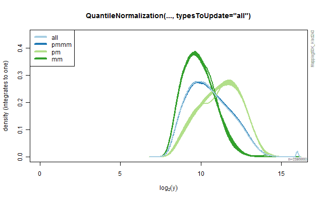
Figure 2A.

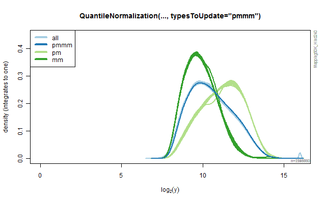
Figure 2B.

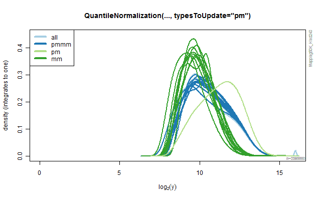
Figure 2C.

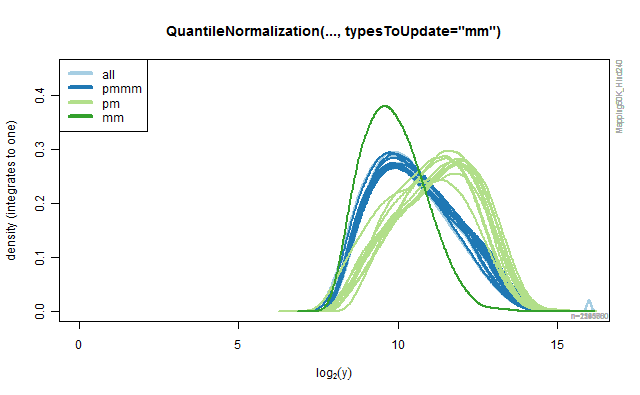
Figure 2D.

for (type in types) {
  verbose && enter(verbose, "Rank-based quantile normalization on ", type, " probes")
  verbose && cat(verbose, "typesToUpdate: ", type)
  qn <- QuantileNormalization(csR, typesToUpdate=type, tags=c("*", type))
  print(qn)
  csN <- process(qn, verbose=verbose)

  toPNG("plotDensity", tags=c("QN", type), aspectRatio=0.618, {
    # Plot the type normalized-by last.
    kks <- match(c(setdiff(types, type), type), types)
    for (kk in kks) {
      plotDensity(csN, types=types[kk], subset=NULL, col=cols[kk], lwd=2, ylim=c(0,0.45), add=(kk != kks[1]));
    }
    legend("topleft", col=cols, lwd=4, types)
    title(sprintf("QuantileNormalization(..., typesToUpdate=\"%s\")", type))
  })

  verbose && exit(verbose)
}