Vignette: Using the GenomeGraphs package with FIRMA
Author: Mark Robinson and Henrik Bengtsson
Created on: 2009-03-28
Last updated: 2011-11-10
This page describes some commands that can be used with the Bioconductor GenomeGraphs package for the plotting of probe-level data for FIRMA (Purdom, Simpson, Robinson, Conboy, Lapuk, and Speed, 2008) analyses of exon array data. These have been adopted from code segments that were borrow from Elizabeth Purdom.
FIRMA results
Assume that we have run FIRMA (cf. vignette 'FIRMA: Human exon array analysis') on a HuEx-1_0-st-v2 exon array data set and that the exon-by-transcript probe-level model (PLM) is available in 'plm'. Then we can retrieve the normalized probe signals and the probe-level FIRMA residuals as:
ds <- getDataSet(plm)
rs <- getResidualSet(plm)
NetAffx annotation data
In order to display the FIRMA estimates along genome, we need some additional annotation data for this particular chip type. Affymetrix provides NetAffx tabular text files containing this information. To retrieve this in the Aroma framework, do:
cdf <- getCdf(plm)
chipType <- getChipType(cdf, fullname=FALSE)
na <- AffymetrixNetAffxCsvFile$byChipType(chipType, pattern=".*.probeset.csv$")
print(na)
AffymetrixNetAffxCsvFile:
Name: HuEx-1_0-st-v2.na24.hg18.probeset
Tags:
Full name: HuEx-1_0-st-v2.na24.hg18.probeset
Pathname: annotationData/chipTypes/HuEx-1_0-st-v2/HuEx-1_0-st-v2.na24.hg18.probeset.csv
File size: 372.75 MB (390859128 bytes)
RAM: 0.02 MB
Number of data rows: NA
Columns [39]: 'probesetId', 'seqname', 'strand', 'start', 'stop',
'probeCount','transcriptClusterId', 'exonId', 'psrId', 'geneAssignment',
'mrnaAssignment', 'crosshybType', 'numberIndependentProbes',
'numberCrossHybProbes', 'numberNonoverlappingProbes', 'level',
'bounded', 'noboundedevidence', 'hasCds', 'fl', 'mrna','est',
'vegagene', 'vegapseudogene', 'ensgene', 'sgpgene', 'exoniphy',
'twinscan', 'geneid', 'genscan', 'genscansubopt', 'mouseFl',
'mouseMrna', 'ratFl', 'ratMrna', 'micrornaregistry', 'rnagene',
'mitomap', 'probesetType'
Number of text lines: NA
This file can be downloaded from Affymetrix, via links available on the chip-type page HuEx-1_0-st-v2.
This annotation file contains a lot of information with respect to Ensembl/GenBank/... identifiers and so on that is not directly relevant to what want to do. Here we are interested in only small subset of these columns; 'probesetId', 'seqname', 'strand', 'transcriptClusterId', 'start' and 'stop'. To read those into a data frame, we do:
colClassPatterns <- c("(probesetId|seqname|strand|transcriptClusterId)"="character", "(start|stop)"=NA)
naData <- readDataFrame(na, colClassPatterns=colPatterns)
dim(naData)

## [1] 1425647       6
Plotting one transcript cluster
Here is a possible set of steps to follow in order to do some plotting
of a particular transcript cluster (e.g. one that corresponds to a
probeset that has been identified by FIRMA). Say you have followed the
steps in the human exon array use-case: you have an object plm which
is your probe level model, you have fit it, calculated the residuals and
have run FIRMA, etc. Now, say you want to plot the normalized data and
residuals in the context on known (say, Ensembl) transcripts for that
gene. Here we will demonstrate on the 33 sample tissue dataset. And,
we happen know that WNK1 has a very interesting kidney-specific
isoform.
Here, we know in advance that the WNK1 transcript cluster is represented on the Human Exon array by the identifier '3400034'. In order to identify the probe (cell) indices for this transcript we do:
# Get the unit index
unitName <- "3400034"
unit <- indexOf(cdf, names=unitName)

# Get the (unit, group, cell) index map
ugcM <- getUnitGroupCellMap(cdf, units=unit, retNames=TRUE)

# Get the cell indices
cells <- ugcM$cell
str(cells)

## int [1:200] 5070870 1796705 5331364 2436977 6478403 5485700 ...
Now we can read the log2 normalized probe signals as well as the log2 FIRMA residuals into matrices:
# Probe signals
y <- extractMatrix(ds, cells=cells, verbose=verbose)
y <- log2(y)

# FIRMA residuals
r <- extractMatrix(rs, cells=cells, verbose=verbose)
r <- log2(r)

nbrOfArrays <- ncol(y)
We will need to know the number of probes from each probeset and we will need to match up to the CSV file in order to gather the genome locations for the transcript of interest:
nbrOfProbesPerExon <- table(ugcM$group)
exonNames <- names(nbrOfProbesPerExon)
nbrOfProbesPerExon <- as.integer(nbrOfProbesPerExon);

naDataJ <- subset(naData, probesetId %in% exonNames)
which results in 53x33 data frame.
We wish to highlight the kidney samples in the plots, by adjusting line widths and line colors. The kidney samples have indices 10, 11 and 12:
lwds <- rep(1, times=nbrOfArrays); lwds[10:12] <- 3
cols <- rep("grey", times=nbrOfArrays); cols[10:12] <- "blue"
The following lines create the ExonArray objects which are GenomeGraphs containers for the data to be plotted:
library("GenomeGraphs")
library("R.devices")
devOptions("png", width=1024)

dp <- DisplayPars(plotMap=FALSE, color=cols, lwd=lwds)

ea1 <- new("ExonArray", intensity=y,
           probeStart=naDataJ$start, probeEnd=naDataJ$stop,
           probeId=exonNames, nProbes=nbrOfProbesPerExon, dp=dp)

ea2 <- new("ExonArray", intensity=r,
           probeStart=naDataJ$start, probeEnd=naDataJ$stop,
           probeId=exonNames, nProbes=nbrOfProbesPerExon, dp=dp)
From the genome locations of the probesets of interest, we can query the BioMart database (using the Bioconductor biomaRt package) for the latest update of transcript annotation for that region:
# Set up BioMart
mart <- useMart(biomart="ensembl", dataset="hsapiens_gene_ensembl")

# Gene region for this transcript
chr <- gsub("chr", "", naDataJ$seqname[1])
range <- range(c(naDataJ$start, naDataJ$stop))
gr <- new("GeneRegion", chromosome=chr, start=range[1], end=range[2], strand=naDataJ$strand[1], biomart=mart)

# Transcript annotations
transcriptIds <- unique(gr@ens[,"ensembl_gene_id"])
tr <- new("Transcript", id=transcriptIds, biomart=mart, dp=DisplayPars(plotId=TRUE))

# Genomic annotations
ga <- new("GenomeAxis", add53=TRUE)
Finally, the gdPlot() function creates the actually figure, as shown
below.
tracks <- list(ea1, ga, ea2, gr, tr)

toPNG(getFullName(plm), tags=unitName, aspectRatio=0.8, {
  gdPlot(tracks)
})
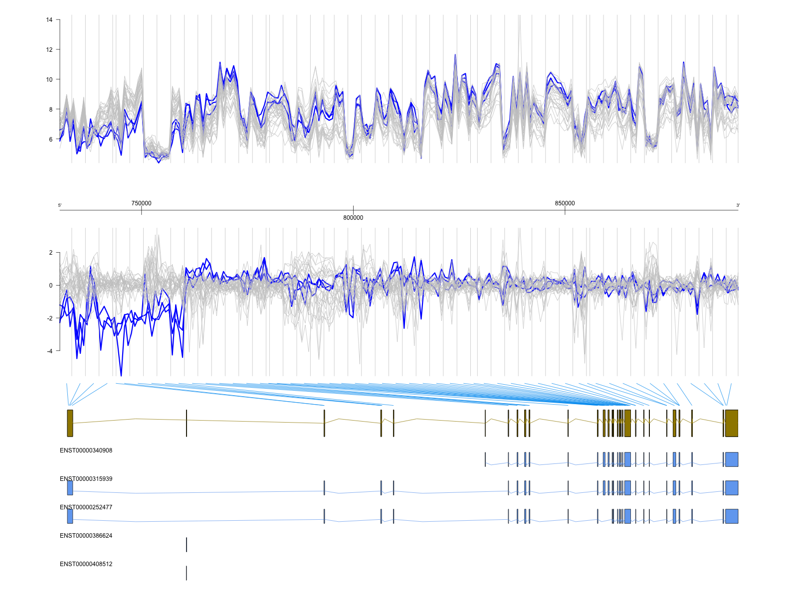
Note of course that most options here are customizable and the user should refer to the GenomeGraphs documentation for all that is available.
References
[1] E. Purdom, K. M. Simpson, M. D. Robinson, et al. "FIRMA: a method for detection of alternative splicing from exon array data". Eng. In: Bioinformatics (Oxford, England) 24.15 (Aug. 2008), pp. 1707-14. ISSN: 1367-4811. DOI: 10.1093/bioinformatics/btn284. PMID: 18573797.