Vignette: Multi-source copy-number normalization (MSCN)
Author: Henrik Bengtsson
Created on: 2009-02-12
Last updated on: 2010-01-07
Figure: Before (top) and after (bottom) MSCN normalization looping over estimates from four different centers. Note how the CN mean levels are the same across platforms after normalization.
Introduction
In this vignette we will show how one can normalize same-sample replicated measurements of copy-number estimates (CNs) originating from different platforms and labs. The normalization method is referred to as multi-source copy-number normalization, or short MSCN (Bengtsson, Ray, Spellman, and Speed, 2009). MSCN is a single-sample method meaning the normalization of one sample is independent of the others, which also means that it can be applied to one sample at the time. The MSCN method normalizes total CNs, that is, if allele-specific estimates exist, the ratio between Allele A and Allele B is preserved, i.e. theta[A]/theta[B] remains unchanged.
Here we will use a small set of tumor-normal log-CNs from The Cancer Genome Atlas (TCGA) project, more precisely we will normalize CNs for samples TCGA-02-0026, TCGA-02-0104, TCGA-06-0129, and TCGA-06-0178.
NOTE: Because of possible privacy issues, we are not sure if we can release the small TCGA data set used in this vignette. This is because within the TCGA project it has been decided that data from SNP platforms (Affymetrix and Illumina) cannot be release because the genotype information is available. Here we only use total CNs, but we are still not sure if that is alright. This is the reason why we do not provide a link to download the example data. An alternative is to use a different data set with CN estimates from multiple platforms. Please email HB (see above) with suggestions of other data sets.
Setting up custom CN data sets
This vignette will not explain to you how to setup your own data set in a similar fashion. For instructions on how to do that, please see Vignette 'Creating binary data files containing copy number estimates'.
Setup
The MSCN method is implemented in the aroma.cn package. The aroma.cn package uses a similar directory setup as the aroma.affymetrix package. This that all data and results are retrieved and stored relative to the current directory. All annotation data should be placed under the annotationData/ directory tree and all raw data should be placed under the rawCnData/ directory tree. The details will be explained below.
There are several advantages of this setup, e.g. the same script will work out of the box everywhere, and it is easier to troubleshoot for you and others. It is useful to know that you should not specify pathnames (absolute or relative) in any scripts. If you find yourself specifying a pathname, then you are most likely not doing the correct thing.
Annotation data
The following set of UGP files needs to be placed in the annotationData/ directory tree exactly (case sensitive!) as as shown:
annotationData/
  chipTypes/
    GenericHuman/
       GenericHuman,100kb,HB20080520.ugp
    HG-CGH-244A/
       HG-CGH-244A,TCGA,HB20080512.ugp
    HumanGenomeCGH244A/
       HumanGenomeCGH244A,Agilent,20070207,HB20080526.ugp
    HumanHap550/
       HumanHap550,TCGA,HB20080512.ugp
    GenomeWideSNP_6/
       GenomeWideSNP_6,na26,HB20080821.ugp
Download: These UGP files can be downloaded from /data/annotationData/chipTypes/.
Details: A UGP file is a Unit Genome Position file which maps loci to chromosomal locations. For further details, see How To page 'Create a Unit Genome Position (UGP) files'. The UGP for chip type 'GenericHuman' is independent of chip type and provides a map of loci placed at 100kb along the human genome. This map is used for estimating CNs at a set of common loci regardless of chip type. These binned CNs at common loci will then be used to estimate the non-linear relationships between platforms. All other UGPs are specific to chip type.
Raw data
The following set of ASB files needs to be placed in the rawCnData/ directory tree exactly (case sensitive!) as shown:
rawCnData/
  TCGA,GBM,testSet,pairs,Broad/
    GenomeWideSNP_6/
      TCGA-02-0026-01Bvs10A,B06vsB06,log2ratio,total.asb
      TCGA-02-0104-01Avs10A,B06vsB06,log2ratio,total.asb
      TCGA-06-0129-01Avs10A,B03vsB03,log2ratio,total.asb
      TCGA-06-0178-01Avs10B,B04vsB04,log2ratio,total.asb

  TCGA,GBM,testSet,pairs,Harvard/
    HumanGenomeCGH244A/
      TCGA-02-0026-01Bvs10A,B07vsB07,log2ratio,total.asb
      TCGA-02-0104-01Avs10A,B07vsB07,log2ratio,total.asb
      TCGA-06-0129-01Avs10A,B06vsB06,log2ratio,total.asb
      TCGA-06-0178-01Avs10B,B04vsB04,log2ratio,total.asb

  TCGA,GBM,testSet,pairs,MSKCC/
    HG-CGH-244A/
      TCGA-02-0026-01Bvs10A,direct,B06,log2ratio,total.asb
      TCGA-02-0104-01Avs10A,direct,B06,log2ratio,total.asb
      TCGA-06-0129-01Avs10A,B03vsB03,log2ratio,total.asb
      TCGA-06-0178-01Avs10B,B04vsB04,log2ratio,total.asb

  TCGA,GBM,testSet,pairs,Stanford/
    HumanHap550/
      TCGA-02-0026-01Bvs10A,B04,log2ratio,total.asb
      TCGA-02-0104-01Avs10A,B04,log2ratio,total.asb
      TCGA-06-0129-01Avs10A,B02,log2ratio,total.asb
      TCGA-06-0178-01Avs10B,B03,log2ratio,total.asb
Download:
These data files can be downloaded from:
Sorry, currently we cannot redistribute this data set. See above note.
Comment on file names:
The above filenames follow a standard outlined by the aroma.affymetrix
project, where a filename consists of a so called name part and comma
separated tags followed by the filename extension. For instance, the
filename 'TCGA-02-0026-01Bvs10A,B04,log2ratio,total.asb' can divided up
in to the name 'TCGA-02-0026-01Bvs10A' followed by the three tags 'B04',
'log2ratio', and 'total'. The filename extension is 'asb'. The name
and the tags together constitutes the so called fullname, e.g.
'TCGA-02-0026-01Bvs10A,B04,log2ratio,total'. Directory names are parsed
similarly.
Important: It is the name part of each filename that specifies the sample name, e.g. 'TCGA-02-0026-01Bvs10A'. The name part is used to identify the set of arrays (hybridizations) across sources that contains CNs for the same sample such that they can be normalized together. The name part must be identical (case sensitive) across sets. As illustrated by the above data files, the tags does not have to match across sources.
Important:
Allele-specific CN estimates cannot be released publicly in the TCGA
project. For this reason, the above data set contains only total CN
estimates.
Example of a complete MSCN script
Before walking through the lengthy details of the MSCN method, the following few lines of code is actually all it takes when using the aroma.cn package:
library("aroma.cn")
log <- Arguments$getVerbose(-8, timestamp=TRUE)
tagsList <- list("MSKCC", "Harvard", "Stanford", "Broad")
dataSet <- "TCGA,GBM,testSet,pairs"
dsList <- lapply(tagsList, FUN=function(tags) {
  AromaUnitTotalCnBinarySet$byName(dataSet, tags=tags, chipType="*")
})
ugp <- AromaUgpFile$byChipType("GenericHuman", tags="100kb")
mscn <- MultiSourceCopyNumberNormalization(dsList, fitUgp=ugp)
dsNList <- process(mscn, verbose=log)
The normalized data is saved to disk under cnData/ in a structure similar to rawCnData/.
Next we will walk through the details of MSCN.
Startup
library("aroma.cn")
log <- Arguments$getVerbose(-8, timestamp=TRUE)
Loading raw CN data set
tagsList <- list("MSKCC", "Harvard", "Stanford", "Broad")
dataSet <- "TCGA,GBM,testSet,pairs"

dsList <- lapply(tagsList, FUN=function(tags) {
  AromaUnitTotalCnBinarySet$byName(dataSet, tags=tags, chipType="*")
})

# Keep only common samples (not needed here, but in other data sets)
names <- Reduce(intersect, lapply(dsList, FUN=getNames))
dsList <- lapply(dsList, FUN=extract, names)
print(dsList)
which lists the "loaded" (they are not really loaded into memory) data sets:
AromaUnitTotalCnBinarySet:
Name: TCGA
Tags: GBM,testSet,pairs,MSKCC
Full name: TCGA,GBM,testSet,pairs,MSKCC
Number of files: 4
Names: TCGA-02-0026-01Bvs10A, TCGA-02-0104-01Avs10A,
TCGA-06-0129-01Avs10A, TCGA-06-0178-01Avs10B
Path (to the first file):
rawCnData/TCGA,GBM,testSet,pairs,MSKCC/HG-CGH-244A
Total file size: 3.60MB
RAM: 0.00MB

[[2]]
AromaUnitTotalCnBinarySet:
Name: TCGA
Tags: GBM,testSet,pairs,Harvard
Full name: TCGA,GBM,testSet,pairs,Harvard
Number of files: 4
Names: TCGA-02-0026-01Bvs10A, TCGA-02-0104-01Avs10A,
TCGA-06-0129-01Avs10A, TCGA-06-0178-01Avs10B
Path (to the first file):
rawCnData/TCGA,GBM,testSet,pairs,Harvard/HumanGenomeCGH244A
Total file size: 3.61MB
RAM: 0.00MB

[[3]]
AromaUnitTotalCnBinarySet:
Name: TCGA
Tags: GBM,testSet,pairs,Stanford
Full name: TCGA,GBM,testSet,pairs,Stanford
Number of files: 4
Names: TCGA-02-0026-01Bvs10A, TCGA-02-0104-01Avs10A,
TCGA-06-0129-01Avs10A, TCGA-06-0178-01Avs10B
Path (to the first file):
rawCnData/TCGA,GBM,testSet,pairs,Stanford/HumanHap550
Total file size: 8.57MB
RAM: 0.00MB

[[4]]
AromaUnitTotalCnBinarySet:
Name: TCGA
Tags: GBM,testSet,pairs,Broad
Full name: TCGA,GBM,testSet,pairs,Broad
Number of files: 4
Names: TCGA-02-0026-01Bvs10A, TCGA-02-0104-01Avs10A,
TCGA-06-0129-01Avs10A, TCGA-06-0178-01Avs10B
Path (to the first file):
rawCnData/TCGA,GBM,testSet,pairs,Broad/GenomeWideSNP_6
Total file size: 28.32MB
RAM: 0.00MB
Note how each of the four data sets contains the same four samples.
Plotting copy numbers
In this section we will show how to plot CNs for a particular sample and genomic region of interest. We will look at the CNs on Chr3:0-60Mb in sample TCGA-02-0104-01Avs10A.
Before we continue, we will set up the sites, platforms and chip types from the data set names, which will be used in the plots. This could have been entered manually, but we are lazy:
tags <- Reduce(intersect, lapply(dsList, FUN=getTags))
sites <- sapply(dsList, FUN=function(ds) setdiff(getTags(ds), tags))
platforms <- sapply(dsList, FUN=getPlatform)
chipTypes <- sapply(dsList, FUN=getChipType)

# Extract (load) CNs in region of interest for the 2nd sample
cnList <- lapply(dsList, FUN=function(ds) {
  df <- ds[[2]]
  extractRawCopyNumbers(df, chromosome=3, region=c(0,60e6))
})
names(cnList) <- paste(sites, platforms, chipTypes, sep=";")
print(cnList)

$`MSKCC;Agilent;HG-CGH-244A`
RawCopyNumbers:
Chromosome: 3
Number of loci: 5376
Loci fields: cn [5376xnumeric], x [5376xnumeric]
RAM: 0.06MB

$`Harvard;Agilent;HumanGenomeCGH244A`
RawCopyNumbers:
Chromosome: 3
Number of loci: 5376
Loci fields: cn [5376xnumeric], x [5376xnumeric]
RAM: 0.06MB

$`Stanford;Illumina;HumanHap550`
RawCopyNumbers:
Chromosome: 3
Number of loci: 12943
Loci fields: cn [12943xnumeric], x [12943xnumeric]
RAM: 0.15MB

$`Broad;Affymetrix;GenomeWideSNP_6`
RawCopyNumbers:
Chromosome: 3
Number of loci: 41279
Loci fields: cn [41279xnumeric], x [41279xnumeric]
RAM: 0.47MB
Note how the four different sources have different number of loci in this region. Since the resolution is different between platforms, it can be very hard to "compare" the different CN estimates, especially if scatter plots are used. To get a better sense of the estimates across platforms, we will also plot smoothed CN estimates by "asking" each platform for its best CN estimates in equally binned 100kb regions (technically we are using contiguous non-overlapping uniform kernel estimators).
# Smooth CNs using consecutive bins of width 100kb
xRange <- range(sapply(cnList, FUN=xRange))
cnSList <- lapply(cnList, FUN=function(cn) {
  binnedSmoothing(cn, from=xRange[1], to=xRange[2], by=100e3)
})
print(cnSList)

$`MSKCC;Agilent;HG-CGH-244A`
RawCopyNumbers:
Chromosome: 3
Number of loci: 600
Loci fields: cn [600xnumeric], x [600xnumeric]
RAM: 0.01MB

$`Harvard;Agilent;HumanGenomeCGH244A`
RawCopyNumbers:
Chromosome: 3
Number of loci: 600
Loci fields: cn [600xnumeric], x [600xnumeric]
RAM: 0.01MB

$`Stanford;Illumina;HumanHap550`
RawCopyNumbers:
Chromosome: 3
Number of loci: 600
Loci fields: cn [600xnumeric], x [600xnumeric]
RAM: 0.01MB

$`Broad;Affymetrix;GenomeWideSNP_6`
RawCopyNumbers:
Chromosome: 3
Number of loci: 600
Loci fields: cn [600xnumeric], x [600xnumeric]
RAM: 0.01MB
Note how these sets of smoothed CNs all consist of the same number of loci. Finally, we will plot the raw and the 100kb-binned CNs for the region of interest:
toPNG("TCGA-02-0104-01Avs10A", tags="rawCNs" width=1024, height=768, {
  Mlim <- c(-3,3)
  layout(seq(along=cnList))
  par(mar=c(4.2,4.2,1.3,2.1), cex=1.1)
  for (kk in seq(along=cnList)) {
    cn <- cnList[[kk]]
    cnS <- cnSList[[kk]]
    plot(cn, ylim=Mlim)
    stext(side=3, pos=0, names(cnList)[kk])
    points(cnS, cex=1, col="white")
    points(cnS, cex=0.5, col="red")
    stext(side=3, pos=1, cex=0.8, sprintf("Chr03 (n=%d; s=%d)", nbrOfLoci(cn), nbrOfLoci(cnS)))
  } # for (kk ...)
})
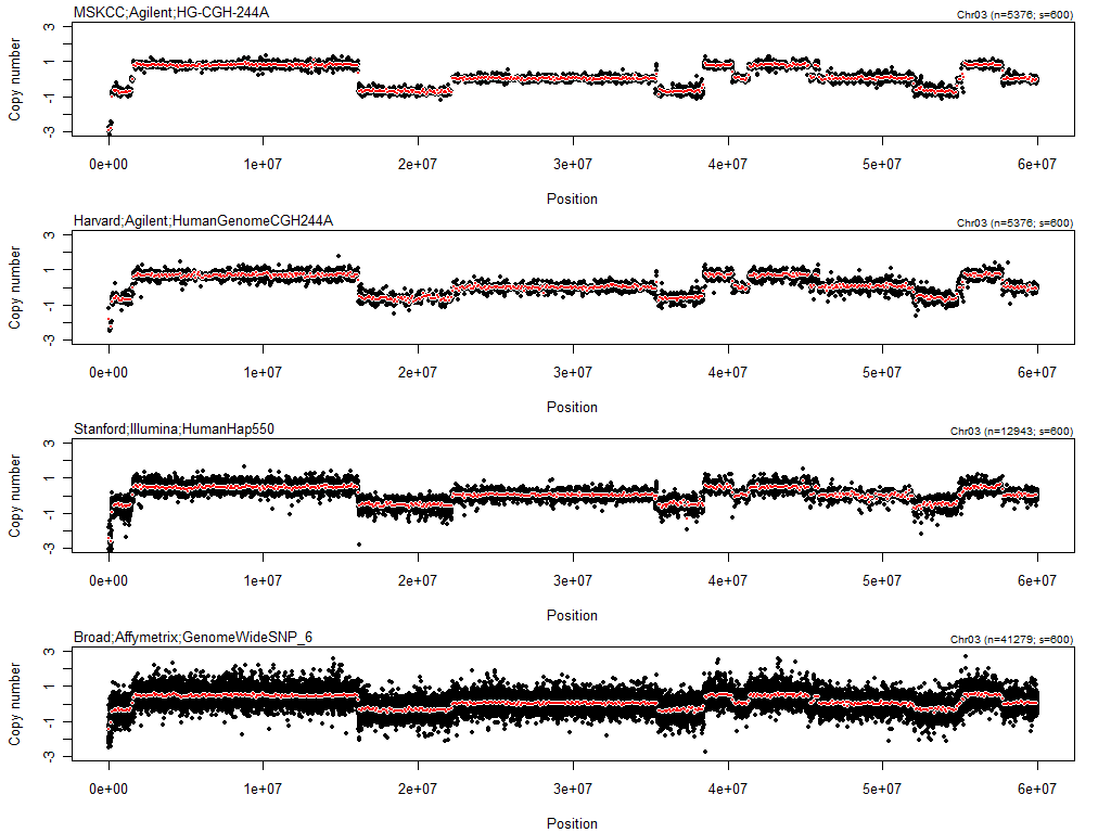
Figure: Raw (black) and 100kb-binned (red) log2 copy-number ratios on Chr3:0-60Mb in TCGA-02-0104-01Avs10A.
To better see the differences between sources, we can plot only smoothed CNs.
toPNG("TCGA-02-0104-01Avs10A", tags="smoothCNs", width=1024, height=320, {
  Mlim <- c(-1.5,1.5)
  par(mar=c(4.2,4.2,1.3,2.1), cex=1.1)
  for (kk in seq(along=cnList)) {
    if (kk == 1) {
      plot(cnSList[[kk]], col=kk, ylim=Mlim)
    } else {
      points(cnSList[[kk]], col=kk)
    }
  } # for (kk ...)
  stext(side=3, pos=1, cex=0.8, sprintf("Chr03 (s=%d)", nbrOfLoci(cnSList[[1]])))
  legend("topleft", pch=19, col=1:4, sites, horiz=TRUE, bty="n")
})
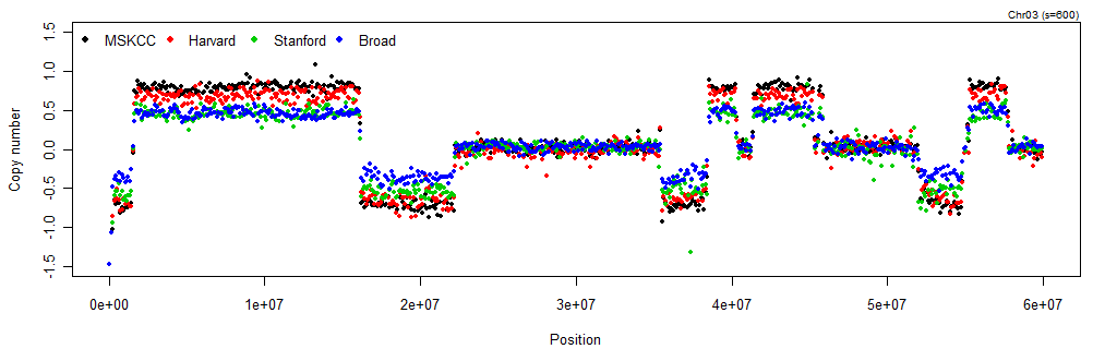
Figure: 100kb-binned log2 copy-number ratios on Chr3:0-60Mb in TCGA-02-0104-01Avs10A according to each of the four sources (labs, platforms, and preprocessing methods). It is clear that for this particular sample, the CN estimates from MSKCC and Harvard (both Agilent) have a greater range than those from Broad (Affymetrix) and Stanford (Illumina). Regardless of differences in amplitude, all four data sets agree strongly on the CN profile.
Normalizing for differences in copy number response functions
When measuring CNs using different techniques such as array-based or next-generation sequencing methods, the estimated CNs are obtained through a sequence of more or less complicated procedures. Many external but also internal factors can affect these steps and the final CN estimates are rarely on the same scale across labs, platforms, and preprocessing methods. For various reasons, they are often not even proportional but rather non linear relative to each other and the underlying truth.
- What the MSCN method does:
- The MSCN method normalizes the full-resolution CN estimates from
different labs and platforms such that they are proportional to each
other, i.e. such that they agree on the CN mean level for any true CN
level.
- The MSCN method normalizes the full-resolution CN estimates from
different labs and platforms such that they are proportional to each
other, i.e. such that they agree on the CN mean level for any true CN
level.
- What the MSCN method does not do:
- The method does not make normalized CN estimates proportional to
the underlying truth. In order to do that, calibration towards a known
truth is needed. However, if one of the sources (data sets) is
calibrated this way or is known to be closer to the truth than the
others, one can specify to normalize toward that set of CNs. The
default is to normalize to the first data set in the list (
dsList). - The method does not normalize for differences in variance levels; dealing with heteroscedasticity is for downstream methods.
- The method does not normalize across samples; it is on purpose a pure single-sample method.
- The method does not make normalized CN estimates proportional to
the underlying truth. In order to do that, calibration towards a known
truth is needed. However, if one of the sources (data sets) is
calibrated this way or is known to be closer to the truth than the
others, one can specify to normalize toward that set of CNs. The
default is to normalize to the first data set in the list (
Smoothed CNs at common loci
In order to normalize CN data sets originating from different platforms with different sets of CN loci, the MSCN method constructs smoothed CN estimates at a common set of loci from the original full-resolution estimates. Here we choose to estimate smoothed CNs at every 100kb along the genome. Neither the distance between nor the exact locations of the common loci is critical. We use a predefine UGP file for specifying the set of common loci used for fitting the CN response functions relative to each other:
ugp <- AromaUgpFile$byChipType("GenericHuman", tags="100kb")
print(ugp)
This display the details of the UGP file to be used:
AromaUgpFile:
Name: GenericHuman
Tags: 100kb,HB20080520
Pathname:
annotationData/chipTypes/GenericHuman/GenericHuman,100kb,HB20080520.ugp
File size: 150.81kB
RAM: 0.00MB
Number of data rows: 30811
File format: v1
Dimensions: 30811x2
Column classes: integer, integer
Number of bytes per column: 1, 4
Footer:
<platform>Generic</platform><chipType>GenericHuman</chipType><createdOn>20080521
10:28:57 PDT</createdOn><createdBy>Henrik Bengtsson,
[email protected]</createdBy><description>A (unit, chromosome,
position) table where units are located every 100kb across the whole
human genome</description>
Chip type: GenericHuman
Platform: Generic
The actual smoothing is done using a truncated Gaussian kernel estimator with a sigma=50kb standard deviation truncated a 3*sigma. The kernel is centered at each target loci. The choice of kernel and bandwidth is not critical either.
Setting up the MSCN method
Next we setup the MSCN method for the four data sets using this set of common loci (this will not perform the normalization, just prepare it):
mscn <- MultiSourceCopyNumberNormalization(dsList, fitUgp=ugp)
print(mscn)
This displays the details of the MSCN to be performed and which data sets that are to be processed:
MultiSourceCopyNumberNormalization:
Data sets (4):
AromaUnitTotalCnBinarySet:
Name: TCGA
Tags: GBM,testSet,pairs,MSKCC
Full name: TCGA,GBM,testSet,pairs,MSKCC
Number of files: 4
Names: TCGA-02-0026-01Bvs10A, TCGA-02-0104-01Avs10A,
TCGA-06-0129-01Avs10A, TCGA
-06-0178-01Avs10B
Path (to the first file):
rawCnData/TCGA,GBM,testSet,pairs,MSKCC/HG-CGH-244A
Total file size: 3.60MB
RAM: 0.00MB
AromaUnitTotalCnBinarySet:
Name: TCGA
Tags: GBM,testSet,pairs,Harvard
Full name: TCGA,GBM,testSet,pairs,Harvard
Number of files: 4
Names: TCGA-02-0026-01Bvs10A, TCGA-02-0104-01Avs10A,
TCGA-06-0129-01Avs10A, TCGA
-06-0178-01Avs10B
Path (to the first file):
rawCnData/TCGA,GBM,testSet,pairs,Harvard/HumanGenomeCGH244A
Total file size: 3.61MB
RAM: 0.00MB
AromaUnitTotalCnBinarySet:
Name: TCGA
Tags: GBM,testSet,pairs,Stanford
Full name: TCGA,GBM,testSet,pairs,Stanford
Number of files: 4
Names: TCGA-02-0026-01Bvs10A, TCGA-02-0104-01Avs10A,
TCGA-06-0129-01Avs10A, TCGA
-06-0178-01Avs10B
Path (to the first file):
rawCnData/TCGA,GBM,testSet,pairs,Stanford/HumanHap550
Total file size: 8.57MB
RAM: 0.00MB
AromaUnitTotalCnBinarySet:
Name: TCGA
Tags: GBM,testSet,pairs,Broad
Full name: TCGA,GBM,testSet,pairs,Broad
Number of files: 4
Names: TCGA-02-0026-01Bvs10A, TCGA-02-0104-01Avs10A,
TCGA-06-0129-01Avs10A, TCGA
-06-0178-01Avs10B
Path (to the first file):
rawCnData/TCGA,GBM,testSet,pairs,Broad/GenomeWideSNP_6
Total file size: 28.32MB
RAM: 0.00MB
Number of common array names: 4
Names: TCGA-02-0026-01Bvs10A, TCGA-02-0104-01Avs10A,
TCGA-06-0129-01Avs10A, TCGA
-06-0178-01Avs10B
Parameters: subsetToFit: int [1:28683] 1 2 3 4 5 6 7 8 9 10 ...
fitUgp:Classes 'AromaUgpFile', 'AromaUnitTabularBinaryFile',
'AromaMicroarrayTabularBinaryFile', 'AromaPlatformInterface',
'AromaTabularBinaryFile', 'GenericTabularFile', 'GenericDataFile',
'Object' atomic [1:1] NA; .. ..- attr(*, ".env")=<environment:
0x03631bd4>; .. ..- attr(*, "...instantiationTime")= POSIXct[1:1],
format: "2009-02-12 19:49:50"; targetDimension: int 1
Note that the MSCN method identified four common array names (actually sample names), namely TCGA-02-0026-01Bvs10A, TCGA-02-0104-01Avs10A, TCGA-06-0129-01Avs10A, and TCGA-06-0178-01Avs10B. This is what we expected. These are the samples for which the full-resolution CN estimates will be normalized across sources.
Conducting the complete normalization procedure
In order to actually perform the normalization, one has to call the
process() method of the normalization object. Since this will take some
time, we tell it to display detailed verbose output while doing it:
dsNList <- process(mscn, verbose=log)
This will perform all steps of the MSCN method internally and output normalized full-resolution CN estimates such that they agree of the CN mean level across all sources (labs, platforms, and preprocessing methods). The output data sets are saved to the cnData/ directory tree
print(dsNList)

[[1]]
AromaUnitTotalCnBinarySet:
Name: TCGA
Tags: GBM,testSet,pairs,MSKCC,mscn
Full name: TCGA,GBM,testSet,pairs,MSKCC,mscn
Number of files: 4
Names: TCGA-02-0026-01Bvs10A, TCGA-02-0104-01Avs10A,
TCGA-06-0129-01Avs10A, TCGA-06-0178-01Avs10B
Path (to the first file):
cnData/TCGA,GBM,testSet,pairs,MSKCC,mscn/HG-CGH-244A
Total file size: 3.60MB
RAM: 0.00MB

[[2]]
AromaUnitTotalCnBinarySet:
Name: TCGA
Tags: GBM,testSet,pairs,Harvard,mscn
Full name: TCGA,GBM,testSet,pairs,Harvard,mscn
Number of files: 4
Names: TCGA-02-0026-01Bvs10A, TCGA-02-0104-01Avs10A,
TCGA-06-0129-01Avs10A, TCGA-06-0178-01Avs10B
Path (to the first file):
cnData/TCGA,GBM,testSet,pairs,Harvard,mscn/HumanGenomeCGH244A
Total file size: 3.61MB
RAM: 0.00MB

[[3]]
AromaUnitTotalCnBinarySet:
Name: TCGA
Tags: GBM,testSet,pairs,Stanford,mscn
Full name: TCGA,GBM,testSet,pairs,Stanford,mscn
Number of files: 4
Names: TCGA-02-0026-01Bvs10A, TCGA-02-0104-01Avs10A,
TCGA-06-0129-01Avs10A, TCGA-06-0178-01Avs10B
Path (to the first file):
cnData/TCGA,GBM,testSet,pairs,Stanford,mscn/HumanHap550
Total file size: 8.57MB
RAM: 0.00MB

[[4]]
AromaUnitTotalCnBinarySet:
Name: TCGA
Tags: GBM,testSet,pairs,Broad,mscn
Full name: TCGA,GBM,testSet,pairs,Broad,mscn
Number of files: 4
Names: TCGA-02-0026-01Bvs10A, TCGA-02-0104-01Avs10A,
TCGA-06-0129-01Avs10A, TCGA-06-0178-01Avs10B
Path (to the first file):
cnData/TCGA,GBM,testSet,pairs,Broad,mscn/GenomeWideSNP_6
Total file size: 28.32MB
RAM: 0.00MB
Note the similarly to the output of the raw data sets (dsList). The
only differences are that a new tag, 'mscn', has been added to each of
the four normalized data set, and that these data sets now are located
under cnData/ whereas before they where located under rawCnData/. If
you look at the cnData/ directory tree, you will find:
cnData/
  TCGA,GBM,testSet,pairs,Broad,mscn/
    GenomeWideSNP_6/
      TCGA-02-0026-01Bvs10A,B06vsB06,log2ratio,total.asb
      TCGA-02-0104-01Avs10A,B06vsB06,log2ratio,total.asb
      TCGA-06-0129-01Avs10A,B03vsB03,log2ratio,total.asb
      TCGA-06-0178-01Avs10B,B04vsB04,log2ratio,total.asb

  TCGA,GBM,testSet,pairs,Harvard,mscn/
    HumanGenomeCGH244A/
      TCGA-02-0026-01Bvs10A,B07vsB07,log2ratio,total.asb
      TCGA-02-0104-01Avs10A,B07vsB07,log2ratio,total.asb
      TCGA-06-0129-01Avs10A,B06vsB06,log2ratio,total.asb
      TCGA-06-0178-01Avs10B,B04vsB04,log2ratio,total.asb

  TCGA,GBM,testSet,pairs,MSKCC,mscn/
    HG-CGH-244A/
      TCGA-02-0026-01Bvs10A,direct,B06,log2ratio,total.asb
      TCGA-02-0104-01Avs10A,direct,B06,log2ratio,total.asb
      TCGA-06-0129-01Avs10A,B03vsB03,log2ratio,total.asb
      TCGA-06-0178-01Avs10B,B04vsB04,log2ratio,total.asb

  TCGA,GBM,testSet,pairs,Stanford,mscn/
    HumanHap550/
      TCGA-02-0026-01Bvs10A,B04,log2ratio,total.asb
      TCGA-02-0104-01Avs10A,B04,log2ratio,total.asb
      TCGA-06-0129-01Avs10A,B02,log2ratio,total.asb
      TCGA-06-0178-01Avs10B,B03,log2ratio,total.asb
Comment on the aroma.cn implementation:
If one calls process() again, the package recognizes that the data has
already been normalized and returned the normalized data sets
momentarily. This is also true, even if one restarts R.
Results
After normalization, all sources agree not only on the copy number profile, but also on the CN mean levels. Similarly to how we did for the raw data set, we will here extract the normalized CNs and plot the smoothed CNs in the same panel.
# Extract normalized CNs in region of interest for the 2nd sample
cnNList <- lapply(dsNList, FUN=function(ds) {
  df <- ds[[2]]
  extractRawCopyNumbers(df, chromosome=3, region=c(0,60e6))
})
names(cnNList) <- paste(sites, platforms, chipTypes, sep=";")

# Smooth CNs using consecutive bins of width 100kb
xRange <- range(sapply(cnNList, FUN=xRange))
cnNSList <- lapply(cnNList, FUN=function(cn) {
  binnedSmoothing(cn, from=xRange[1], to=xRange[2], by=100e3)
})

toPNG("TCGA-02-0104-01Avs10A", tags="mscn,smoothCNs", width=1024, height=320, {
  Mlim <- c(-1.5,1.5)
  par(mar=c(4.2,4.2,1.3,2.1), cex=1.1)
  for (kk in seq(along=cnNSList)) {
    if (kk == 1) {
      plot(cnNSList[[kk]], col=kk, ylim=Mlim)
    } else {
      points(cnNSList[[kk]], col=kk)
    }
  }
  stext(side=3, pos=1, cex=0.8, sprintf("Chr03 (s=%d)", nbrOfLoci(cnNSList[[1]])))
  legend("topleft", pch=19, col=1:4, sites, horiz=TRUE, bty="n")
})
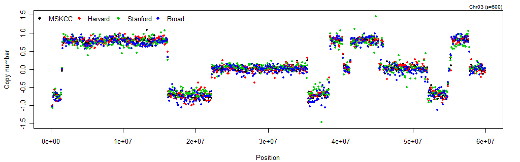
Figure: The copy-number estimates agree across sources after applying normalizing the (full-resolution) MSCN method.
All intermediate and final results are saved to the file system. For
instance, the smoothed CNs used internally for estimating the
relationships between sources are stored in the smoothCnData/ directory
tree. Although it is rarely the case that one wish to work with the
smoothed data sets, these can be retrieved easily be retrieved from the
mscn object. We will here use the smoothed CN estimates to illustrate
the non-linear relationships between sources. This code snippet also
show how to access the data.
dsSList <- getSmoothedDataSets(mscn)

# Identify all (28,683)  units on Chr1-22
units <- getUnitsOnChromosomes(ugp, 1:22)

# Extract CN estimates for these across all data sets in the 2nd sample
M <- sapply(dsSList, FUN=function(dsS) {
  df <- dsS[[2]]
  extractMatrix(df, units=units)
})
colnames(M) <- paste(sites, platforms, chipTypes, sep="\n")

toPNG("TCGA-02-0104-01Avs10A", tags="smoothCNs,pairs", width=640, height=640, {
  par(mar=c(4.2,4.2,1.3,2.1), cex=1.1)
  Mlim <- c(-1.5,1.5)
  panel <- function(...) { abline(a=0, b=1, lty=2); points(...); }
  pairs(M, pch=20, col="red", lower.panel=NULL, upper.panel=panel, xlim=Mlim, ylim=Mlim)
})
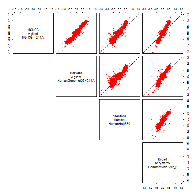
Figure: Non-linear relationships of smoothed copy numbers before normalization.
In order to display the corresponding relationships for the normalized data, we first have to generate smoothed CNs based on the normalized data. The easiest way to achieve this is to "fool" aroma.cn to think we want to apply a 2nd round of MSCN on the normalized data
mscn2 <- MultiSourceCopyNumberNormalization(dsNList, fitUgp=ugp)
However, instead of starting the normalization, we will only ask for the smooth data by:
dsNSList <- getSmoothedDataSets(mscn2, verbose=log)
This will generate the smoothed normalized CN estimates (the output will be stored in smoothCnData/ with data sets containing tag 'mscn'). When the above procedure finishes, we extract the CN estimates as before:
MN <- sapply(dsNSList, FUN=function(dsS) {
  df <- dsS[[2]]
  extractMatrix(df, units=units)
})
colnames(MN) <- paste(sites, platforms, chipTypes, sep="\n")

toPNG("TCGA-02-0104-01Avs10A", tags="mscn,smoothCNs,pairs", width=640, height=640, {
  par(mar=c(4.2,4.2,1.3,2.1), cex=1.1)
  Mlim <- c(-1.5,1.5)
  panel <- function(...) { abline(a=0, b=1, lty=2); points(...); }
  pairs(MN, pch=20, col="red", lower.panel=NULL, upper.panel=panel, xlim=Mlim, ylim=Mlim)
})
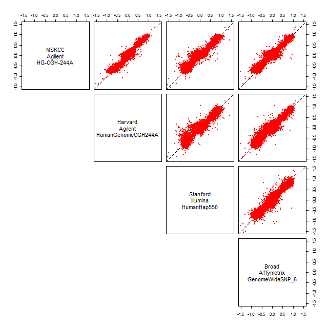
Figure: Linear relationships (on the same scale) of smoothed copy numbers after normalization.
References
[1] H. Bengtsson, A. Ray, P. Spellman, et al. "A single-sample method for normalizing and combining full-resolution copy numbers from multiple platforms, labs and analysis methods". Eng. In: Bioinformatics (Oxford, England) 25.7 (Apr. 2009), pp. 861-7. ISSN: 1367-4811. DOI: 10.1093/bioinformatics/btp074. PMID: 19193730.
Appendix
Comments on processing speed:
Currently MSCN is spending most of its time in generating the smoothed
CN estimates. The smoothing is done using a kernel estimator
implemented in plain R. It is rather likely that one can optimize this
estimator further and even more so by providing a native-code
implementation. Contributions or comments are appreciated.
Low-level functions: The basic low-level functions involved for smoothing, fitting, and normalizing the data according to MSCN are:
- Smoothing:
kernelSmoothing()in aroma.core. - Fitting S-dimensional principal curve:
fitPrincipalCurve()in aroma.light. - Normalization:
backtransformPrincipalCurve()in aroma.light.