Vignette: CalMaTe - A calibration method to improve allele-specific copy number of SNP arrays for downstream segmentation
Created on: 2010-07-30
Last updated: 2014-12-21
Introduction
CalMaTe calibrates preprocessed allele-specific copy-number estimates (ASCNs) from DNA microarrays by controlling for SNP-specific allelic crosstalk. The resulting ASCNs are on average more accurate, which increases the power of segmentation methods (e.g. PSCBS by Olshen, Bengtsson, Neuvial, Spellman, Olshen, and Seshan (2011)) for detecting changes between copy-number states in tumor studies including copy-neutral loss of heterozygosity (LOH). CalMaTe applies to any ASCNs regardless of preprocessing method and microarray technology, e.g. Affymetrix and Illumina. Contrary to the TumorBoost (Bengtsson, Neuvial, and Speed, 2010), which requires a single pair of tumor-normal samples, the CalMaTe methods don't require matched normals, but instead it requires a large number of reference samples. For more details, see Ortiz-Estevez, Aramburu, Bengtsson, Neuvial, and Rubio (2012).
Data
Below we will use the public GEO data set GSE12702:
rawData/
   GSE12702/
     Mapping250K_Nsp/
       GSM318728.CEL, GSM318729.CEL, ..., GSM318767.CEL
Analysis
Allele-specific copy-number estimation (CRMA v2)
We will use an allele-specific version of the CRMA v2 method (Bengtsson, Wirapati, and Speed, 2009) to estimate allele-specific copy numbers (ASCNs) at each SNP. The CRMA v2 method is implemented in the aroma.affymetrix package and the CalMaTe method in the calmate package.
library("aroma.affymetrix")
library("calmate")
verbose <- Arguments$getVerbose(-8, timestamp=TRUE)

# Setting up data set
csR <- AffymetrixCelSet$byName("GSE12702", chipType="Mapping250K_Nsp")
print(csR)

## AffymetrixCelSet:
## Name: GSE12702
## Tags:
## Path: rawData/GSE12702/Mapping250K_Nsp
## Platform: Affymetrix
## Chip type: Mapping250K_Nsp
## Number of arrays: 40
## Names: GSM318728, GSM318729, ..., GSM318767
## Time period: 2008-04-03 13:52:53 -- 2008-04-10 20:08:49
## Total file size: 2506.11MB
## RAM: 0.06MB


# Allele-specific CRMA v2 with log-additive modeling
dsList <- doASCRMAv2(csR, plm="RmaCnPlm", verbose=verbose)
print(dsList)

## $total
## AromaUnitTotalCnBinarySet:
## Name: GSE12702
## Tags: ACC,-XY,BPN,-XY,RMA,FLN,-XY
## Full name: GSE12702,ACC,-XY,BPN,-XY,RMA,FLN,-XY
## Number of files: 40
## Names: GSM318728, GSM318729, ..., GSM318767 [40]
## Path (to the first file): totalAndFracBData/GSE12702,ACC,-XY,BPN,-XY,RMA,FLN,-XY/Mapping250K_Nsp
## Total file size: 40.05 MB
## RAM: 0.06MB##
## $fracB
## AromaUnitFracBCnBinarySet:
## Name: GSE12702
## Tags: ACC,-XY,BPN,-XY,RMA,FLN,-XY
## Full name: GSE12702,ACC,-XY,BPN,-XY,RMA,FLN,-XY
## Number of files: 40
## Names: GSM318728, GSM318729, ..., GSM318767 [40]
## Path (to the first file): totalAndFracBData/GSE12702,ACC,-XY,BPN,-XY,RMA,FLN,-XY/Mapping250K_Nsp
## Total file size: 40.05 MB
## RAM: 0.05MB
Calibration of ASCN estimates (CalMaTe)
cmt <- CalMaTeCalibration(dsList)
print(cmt)

## CalMaTeCalibration:
## Data sets (2):
## <Total>:
## AromaUnitTotalCnBinarySet:
## Name: GSE12702
## Tags: ACC,-XY,BPN,-XY,RMA,FLN,-XY
## Full name: GSE12702,ACC,-XY,BPN,-XY,RMA,FLN,-XY
## Number of files: 40
## Names: GSM318728, GSM318729, ..., GSM318767 [40]
## Path (to the first file): totalAndFracBData/GSE12702,ACC,-XY,BPN,-XY,RMA,FLN,-XY/Mapping250K_Nsp
## Total file size: 40.05 MB
## RAM: 0.06MB
## <FracB>:
## AromaUnitFracBCnBinarySet:
## Name: GSE12702
## Tags: ACC,-XY,BPN,-XY,RMA,FLN,-XY
## Full name: GSE12702,ACC,-XY,BPN,-XY,RMA,FLN,-XY
## Number of files: 40
## Names: GSM318728, GSM318729, ..., GSM318767 [40]
## Path (to the first file): totalAndFracBData/GSE12702,ACC,-XY,BPN,-XY,RMA,FLN,-XY/Mapping250K_Nsp
## Total file size: 40.05 MB
## RAM: 0.05MB

dsCList <- process(cmt, verbose=verbose)
print(dsCList)

## $total
## AromaUnitTotalCnBinarySet:
## Name: GSE12702
## Tags: ACC,-XY,BPN,-XY,RMA,FLN,-XY,CMTN
## Full name: GSE12702,ACC,-XY,BPN,-XY,RMA,FLN,-XY,CMTN
## Number of files: 40
## Names: GSM318728, GSM318729, ..., GSM318767 [40]
## Path (to the first file): totalAndFracBData/GSE12702,ACC,-XY,BPN,-XY,RMA,FLN,-XY,CMTN/Mapping250K_Nsp
## Total file size: 40.05 MB
## RAM: 0.06MB
##
## $fracB
## AromaUnitFracBCnBinarySet:
## Name: GSE12702
## Tags: ACC,-XY,BPN,-XY,RMA,FLN,-XY,CMTN
## Full name: GSE12702,ACC,-XY,BPN,-XY,RMA,FLN,-XY,CMTN
## Number of files: 40
## Names: GSM318728, GSM318729, ..., GSM318767 [40]
## Path (to the first file): totalAndFracBData/GSE12702,ACC,-XY,BPN,-XY,RMA,FLN,-XY,CMTN/Mapping250K_Nsp
## Total file size: 40.05 MB
## RAM: 0.05MB
CalMaTe calibration using only a subset of the data set as references
As this particular data sets consists of tumor and normal samples, it may be advantageous to use only normal samples for the calibration step (and then backtransform all arrays using the estimated calibration). First we identify the indices of the samples that should be used as references:
names <- getNames(dsList$total)

patientIDs <- c(24, 25, 27, 31, 45, 52, 58, 60, 75, 110, 115, 122, 128, 137, 138, 140, 154, 167, 80, 96)
sampleTypes <- c("tumor", "normal")

pids <- rep(patientIDs, each=length(sampleTypes))
types <- rep(sampleTypes, times=length(patientIDs))

mat <- cbind(names, pids, types)
str(mat)
## chr [1:40, 1:3] "GSM318728" "GSM318729" "GSM318730" "GSM318731" ...
##  - attr(*, "dimnames")=List of 2
##   ..$ : NULL
##   ..$ : chr [1:3] "names" "pids" "types"

idxsN <- which(mat[, "types"] == "normal")
Next, when setting up the CalMaTe model, we specify the reference
samples using argument references as follows:
cmtN <- CalMaTeCalibration(dsList, tags=c("*", "normalReferences"), references=idxsN)
print(cmtN)

## CalMaTeCalibration:
##   Data sets (2):
##   <Total>:
##   AromaUnitTotalCnBinarySet:
##   Name: GSE12702
## Tags: ACC,-XY,BPN,-XY,RMA,FLN,-XY
## Full name: GSE12702,ACC,-XY,BPN,-XY,RMA,FLN,-XY
## Number of files: 40
## Names: GSM318728, GSM318729, ..., GSM318767 [40]
## Path (to the first file): totalAndFracBData/GSE12702,ACC,-XY,BPN,-XY,RMA,FLN,-XY/Mapping250K_Nsp
## Total file size: 40.05 MB
## RAM: 0.06MB
## <FracB>:
##   AromaUnitFracBCnBinarySet:
##   Name: GSE12702
## Tags: ACC,-XY,BPN,-XY,RMA,FLN,-XY
## Full name: GSE12702,ACC,-XY,BPN,-XY,RMA,FLN,-XY
## Number of files: 40
## Names: GSM318728, GSM318729, ..., GSM318767 [40]
## Path (to the first file): totalAndFracBData/GSE12702,ACC,-XY,BPN,-XY,RMA,FLN,-XY/Mapping250K_Nsp
## Total file size: 40.05 MB
## RAM: 0.05MB

dsCNList <- process(cmtN, verbose=verbose)
print(dsCNList)

## $total
## AromaUnitTotalCnBinarySet:
## Name: GSE12702
## Tags: ACC,-XY,BPN,-XY,RMA,FLN,-XY,CMTN,normalReferences
## Full name: GSE12702,ACC,-XY,BPN,-XY,RMA,FLN,-XY,CMTN,normalReferences
## Number of files: 40
## Names: GSM318728, GSM318729, ..., GSM318767 [40]
## Path (to the first file): totalAndFracBData/GSE12702,ACC,-XY,BPN,-XY,RMA,FLN,-XY,CMTN,normalReferences/Mapping250K_Nsp
## Total file size: 40.05 MB
## RAM: 0.06MB

## $fracB
## AromaUnitFracBCnBinarySet:
## Name: GSE12702
## Tags: ACC,-XY,BPN,-XY,RMA,FLN,-XY,CMTN,normalReferences
## Full name: GSE12702,ACC,-XY,BPN,-XY,RMA,FLN,-XY,CMTN,normalReferences
## Number of files: 40
## Names: GSM318728, GSM318729, ..., GSM318767 [40]
## Path (to the first file): totalAndFracBData/GSE12702,ACC,-XY,BPN,-XY,RMA,FLN,-XY,CMTN,normalReferences/Mapping250K_Nsp
## Total file size: 40.05
## RAM: 0.05MB
Results
extractSignals <- function(dsList, sampleName, reference=c("none", "median"), refIdxs=NULL, ..., verbose=FALSE) {
    reference <- match.arg(reference)
      idx <- indexOf(dsList$total, sampleName)
      dfT <- dsList$total[[idx]]
      dfB <- dsList$fracB[[idx]]
      tcn <- extractRawCopyNumbers(dfT, logBase=NULL, ..., verbose=verbose)
      baf <- extractRawAlleleBFractions(dfB, ..., verbose=verbose)
      if (reference == "median") {
        if (!is.null(refIdxs)) {
          dsR <- dsList$total[refIdxs]
        } else {
          dsR <- dsList$total
        }
        dfTR <- getAverageFile(dsR, verbose=verbose)
        tcnR <- extractRawCopyNumbers(dfTR, logBase=NULL, ..., verbose=verbose)
        tcn <- divideBy(tcn, tcnR)
        setSignals(tcn, 2*getSignals(tcn))
      }
    list(tcn=tcn, baf=baf)
} # extractSignals()

sampleName <- "GSM318736"

pch <- 19
cex <- 0.8

snT <- sampleName
chr <- 8

for (normalRefs in c(TRUE, FALSE)) {
  if (normalRefs) {
    figName <- sprintf("%s,Chr%02d,CalMaTe,normalReferences", snT, chr)
    dataT <- extractSignals(dsList, sampleName=snT, chromosome=chr, reference="median", refIdxs=idxsN, verbose=verbose)
    dataTC <- extractSignals(dsCNList, sampleName=snT, chromosome=chr, verbose=verbose)
  } else {
    figName <- sprintf("%s,Chr%02d,CalMaTe", snT, chr)
    dataT <- extractSignals(dsList, sampleName=snT, chromosome=chr, reference="median", verbose=verbose)
    dataTC <- extractSignals(dsCList, sampleName=snT, chromosome=chr, verbose=verbose)
  }


  toPNG(figName, width=1200, {
    subplots(4, ncol=1)
    par(mar=c(2,5,1,1)+0.1, cex=cex, cex.lab=2.4, cex.axis=2.2)

    plot(dataT$tcn, ylim=c(0,4), pch=pch)
    plot(dataT$baf, pch=pch)
    plot(dataTC$tcn, ylim=c(0,4), pch=pch)
    plot(dataTC$baf, pch=pch)
  })
}
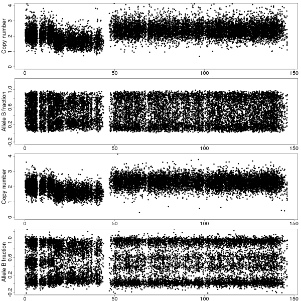
Figure 1a: TCNs and BAFs along chromosome 8 of sample GSM318736 with and without CalMaTe when using all 40 samples are used for calibration. Data is from CRMA v2-processed Affymetrix Mapping250K_Nsp arrays. Top two panels show the TCNs and BAFs before CalMaTe. Bottom two panels show the TCNs and BAFs after CalMaTe. The non-calibrated BAFs are noisy and biased (homozygous clouds are notat 0 and 1) whereas the CalMaTe-calibrated BAFs are much less noisy and located closer to the expected locations. We find that there are three regions, a normal region at 0-20Mb with 2 copies and BAFs near 0, 1/2 and 1 (corresponding to AA, AB and BB genotypes), a deletion at 20-44Mb with1 copy and BAFs close to 0 and 1 (A and B), and a gain at 49-145Mb with 3 copies and BAFs near 0, 1/3, 2/3, and 1 (AAA, AAB, ABB and BBB). The BAFs in the deleted region are noisier because of weaker ASCNs.
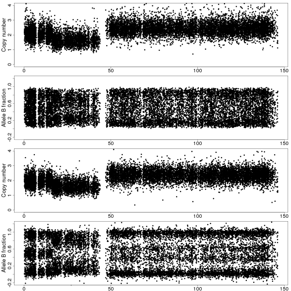
Figure 1b: TCNs and BAFs along chromosome 8 of sample GSM318736 with and without CalMaTe when using all 40 samples are used for calibration. Same data as in Figure 1a. Top two panels show the TCNs and BAFs before CalMaTe. Bottom two panels show the TCNs and BAFs after CalMaTe.
(betaN, betaT) plots
Another way to visualize the effect of CalMaTe on allelic signals, and connect/contrast it with TumorBoost, is to look at tumor-normal pairs and compare allele B fraction in the tumor to allele B fraction in the normal, before and after CalMaTe and/or TumorBoost.
mm <- match(sampleName, names)
id <- pid[mm]

idxT <- which((pid==id) & (type=="tumor"))
snT <- names[idxT]
stopifnot(snT==sampleName)

idxN <- which((pid==id) & (type=="normal"))
snN <- names[idxN]

xlab <- "Normal BAF"
ylab <- "TumorBAF"
lim <- c(-0.1, 1.1)
cext <- 1.8

regions <- list("normal (1,1)"=c(0, 16), "loss (0,1)"=c(16.5, 45), "gain (1,2)"=c(45, 150))

for (rr in seq(along=regions)) {
  reg <- regions[[rr]]
  regLab <- paste(reg, collapse="-")
  cnLab <- names(regions)[rr]
  datT <- extractSignals(dsList, sampleName=snT, chromosome=chr, reg=reg*1e6, verbose=verbose)
  datN <- extractSignals(dsList, sampleName=snN, chromosome=chr, reg=reg*1e6, verbose=verbose)

  datCT <- extractSignals(dsCList, sampleName=snT, chromosome=chr, reg=reg*1e6, verbose=verbose)
  datCN <- extractSignals(dsCList, sampleName=snN, chromosome=chr, reg=reg*1e6, verbose=verbose)

  tbn <- normalizeTumorBoost(datT$baf$y, datN$baf$y, verbose=verbose)
  tbnC <- normalizeTumorBoost(datCT$baf$y, datCN$baf$y, verbose=verbose)

  figName <- sprintf("%s,betaNvsBetaT,Chr%02d,%s", snT, chr, regLab)
  toPNG(figName, width=1200, {
    subplots(4, ncol=2)
    par(mar=c(5,5,2,1)+0.1, cex=cex, cex.lab=2.4, cex.axis=2.2)
    plot(datN$baf$y, datT$baf$y, pch=pch, xlim=lim, ylim=lim, xlab=xlab, ylab=ylab)
    stext("ASCRMAv2", side=3, pos=1, cex=cext)
    stext(cnLab, side=3, pos=0, cex=cext)
    plot(datCN$baf$y, datCT$baf$y, pch=pch, xlim=lim, ylim=lim, xlab=xlab, ylab=ylab)
    stext("ASCRMAv2 + CalMaTe", side=3, pos=1, cex=cext)
    stext(cnLab, side=3, pos=0, cex=cext)
    plot(datN$baf$y, tbn, pch=pch, xlim=lim, ylim=lim, xlab=xlab, ylab=ylab)
    stext("ASCRMAv2 + TumorBoost", side=3, pos=1, cex=cext)
    stext(cnLab, side=3, pos=0, cex=cext)
    plot(datCN$baf$y, tbnC, pch=pch, xlim=lim, ylim=lim, xlab=xlab, ylab=ylab)
    stext("ASCRMAv2 + CalMaTe + TumorBoost", side=3, pos=1, cex=cext)
    stext(cnLab, side=3, pos=0, cex=cext)
  })
}
In Figures 2-4, paired tumor-normal BAFs for three (manually identified) copy number regions on chromosome 8 of sample GSM318736 are displayed for each of the following four combinations of preprocessing methods: ASCRMA v2 (top left), ASCRMA v2 + CalMaTe (top right), ASCRMA v2 + TumorBoost (bottom left), ASCRMA v2 + CalMaTe + TumorBoost (bottom right).
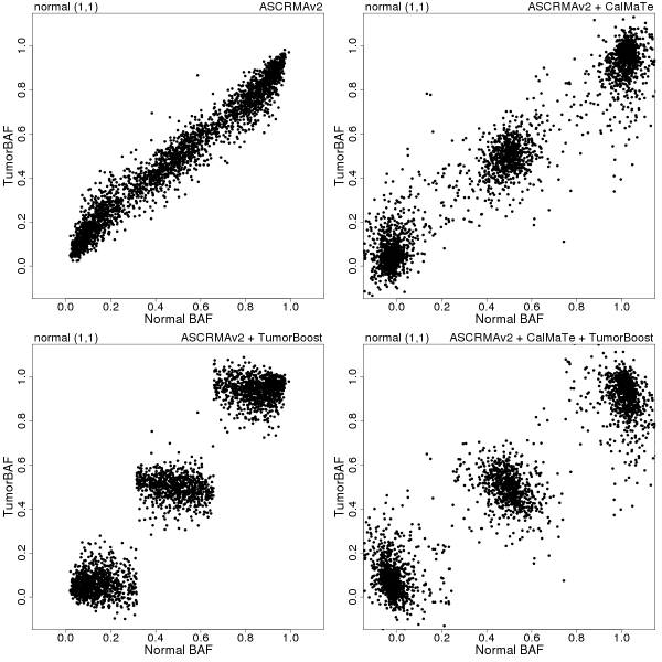
Figure 2: betaT vs betaN in a normal (1,1) region between 0 and 16 Mb on Chromosome 8. Preprocessing methods used: ASCRMA v2 (top left), ASCRMA v2 + CalMaTe (top right), ASCRMA v2 + TumorBoost (bottom left), ASCRMA v2 + CalMaTe + TumorBoost (bottom right).
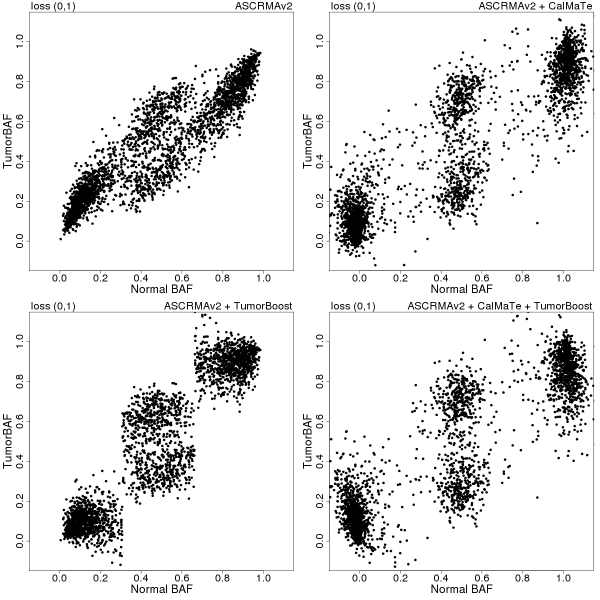
Figure 3: betaT vs betaN in a region of homozygous deletion (0,1) between 16 and 45 Mb on Chromosome 8. Preprocessing methods used: ASCRMA v2 (top left), ASCRMA v2 + CalMaTe (top right), ASCRMA v2 + TumorBoost (bottom left), ASCRMA v2 + CalMaTe + TumorBoost (bottom right).
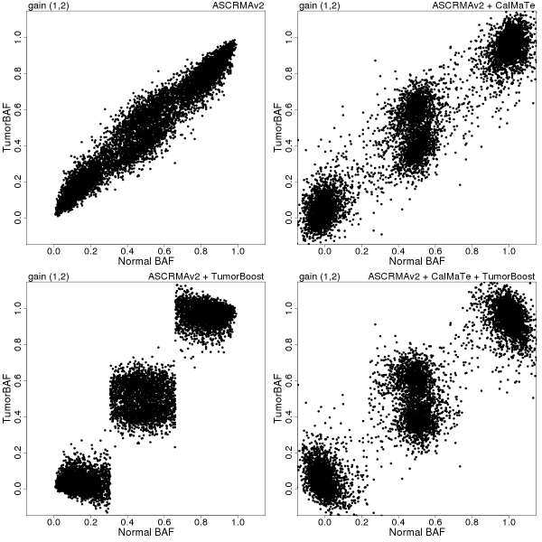
Figure 4: betaT vs betaN in a region of gain (1,2) after 45 Mb on Chromosome 8. Preprocessing methods used: ASCRMA v2 (top left), ASCRMA v2 + CalMaTe (top right), ASCRMA v2 + TumorBoost (bottom left), ASCRMA v2 + CalMaTe + TumorBoost (bottom right).
Note: when comparing signals from TumorBoost to CalMaTe, it is useful to keep in mind that TumorBoost does not normalize the normal sample, whereas CalMaTe calibrates all samples regardless of their types. This means that only the y axes are comparable across the 4 plots. Also, one should focus on SNPs that are heterozygous in the normal samples (they correspond to normal BAFs close to 1/2) as in theory, only these SNPs are informative in terms of copy number changes.
References
[1] H. Bengtsson, P. Wirapati, and T. P. Speed. "A single-array preprocessing method for estimating full-resolution raw copy numbers from all Affymetrix genotyping arrays including GenomeWideSNP 5 & 6". Eng. In: Bioinformatics (Oxford, England) 25.17 (Sep. 2009), pp. 2149-56. ISSN: 1367-4811. DOI: 10.1093/bioinformatics/btp371. PMID: 19535535.
[2] H. Bengtsson, P. Neuvial, and T. P. Speed. "TumorBoost: normalization of allele-specific tumor copy numbers from a single pair of tumor-normal genotyping microarrays". Eng. In: BMC bioinformatics 11 (May. 2010), p. 245. ISSN: 1471-2105. DOI: 10.1186/1471-2105-11-245. PMID: 20462408.
[3] A. B. Olshen, H. Bengtsson, P. Neuvial, et al. "Parent-specific copy number in paired tumor-normal studies using circular binary segmentation". Eng. In: Bioinformatics (Oxford, England) 27.15 (Aug. 2011), pp. 2038-46. ISSN: 1367-4811. DOI: 10.1093/bioinformatics/btr329. PMID: 21666266.
[4] M. Ortiz-Estevez, A. Aramburu, H. Bengtsson, et al. "CalMaTe: a method and software to improve allele-specific copy number of SNP arrays for downstream segmentation". Eng. In: Bioinformatics (Oxford, England) 28.13 (Jul. 2012), pp. 1793-4. ISSN: 1367-4811. DOI: 10.1093/bioinformatics/bts248. PMID: 22576175.